17.4 Introducing the Multi-level VAR
We are often in the situation where we collect intensive longitudinal data on multiple individuals.
Fitting VAR(1) models for every individual in the sample is certainly an option.
However, this can create a large amount of information to summarize and may lead to the recovery of spurious relations depending on how many observations are available for each subject.
One option to consider in this scenario is the multi-level VAR model.
In the multi-level VAR we have the option for each parameter to follow a distribution across individuals. Typically, parameters are expected to follow normal distribution.
Distribution of Parameters
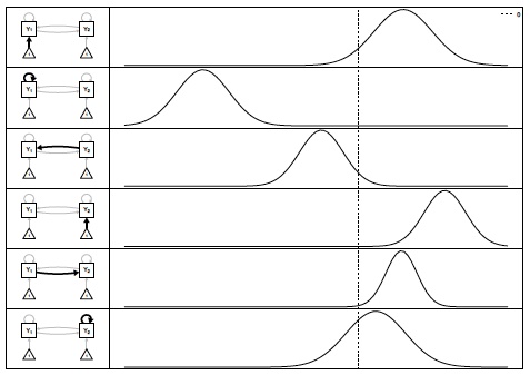
Example Individuals
17.4.1 Model
Now, for illustrative purposes we will use the mlVAR package to demonstrate how one can estimate multi-level VAR models. However, one should note the modeling approach taken in themlVAR package is unique and differs from what we have discussed in class.
For example, themlVAR package also estimates a contemporaneous network following the initial multi-level estimation procedure. We will cover the basics of these routines but one should consults Epskamp, Waldrop, Mottus and Borsboom (2018) for a detailed explanation of the modeling procedures.
The first-stage model can be written as
\[ \mathbf{y}_{t,p} = \boldsymbol{\mu}_{p} + \mathbf{B}_{p}(\mathbf{y}_{t,p}-\boldsymbol{\mu}_{p}) +\boldsymbol{\varepsilon}_{t,p} \]
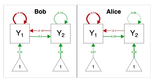
where \(\boldsymbol{\varepsilon}_{t,p} \sim \mathcal{N}(\mathbf{0},\boldsymbol{\theta}_{p})\) and \(\boldsymbol{\theta}_{p}^{-1}=\mathbf{K}_{p}^{(\Theta)}\). Here, \(\boldsymbol{\mu}_{p}\) is the mean vector for subject \(p\), \(\mathbf{B}_{p}\) is the person-specific transition matrix, and \(\mathbf{K}_{p}\) is the person-specific contemporaneous relations.
Unfortunately, many multi-level software routines will be unable to estimate \(\boldsymbol{\mu}_{p}\) in a straightforward manner. In accordance with Hamaker & Grasman (2014) and Epskamp et al. (2018) one possibility is to use \(\bar{\mathbf{y}}_{p}\) in place of \(\boldsymbol{\mu}_{p}\). This simplication allows us to estimate the VAR model as a series of univariate regressions (within-subject centered predictors) using generic multi-level software such as nlme or lme4.
In this context the Level 1 model can be written as
\[ y_{t,p,i} = \mu_{p,i} + \mathbf{B}_{p,i}(\mathbf{y}_{t-1,p}-\bar{\mathbf{y}}_{p}) +\varepsilon_{t,p,i} \]
and the Level 2 model as
\[ \left[ \begin{array}{c} \mu_{p,i} \\ B_{p,i} \end{array} \right] \sim \mathcal{N} \left[ \begin{array}{c} \mathbf{0} \\ B_{*,i} \end{array} \right], \left[ \begin{array}{cc} \omega_{\mu_{i}} & \boldsymbol{\omega}^{(\beta_{i}\mu_{i})'}\\ \boldsymbol{\omega}^{(\beta_{i}\mu_{i})} & \boldsymbol{\Omega}^{(\mathbf{B}_{i})} \end{array} \right] \]
where \(\mathbf{B}_{*}\) and \(\mathbf{K}_{*}^{(\Theta)}\) represent the temporal and contemporaneous network for a person selected at random, or the average parameters in the population: the fixed effects.