13.3 Individual Growth Models

To introduce growth modeling we will begin with data from a single individual. Let’s make a dataset with just 1 person of interest, id = 23,

verb_id23 <- verblong[which(verblong$id == 23), ]

13.3.1 Visualizing Individual Change

Let’s make a plot of this person’s data,

ggplot(data = verb_id23, aes(x = grade, y = verb, group = id)) +
  geom_point() + 
  xlab("Grade") + 
  ylab("WISC Verbal Score") + ylim(0,100) +
  scale_x_continuous(breaks=seq(1,6,by=1)) +
  theme_classic()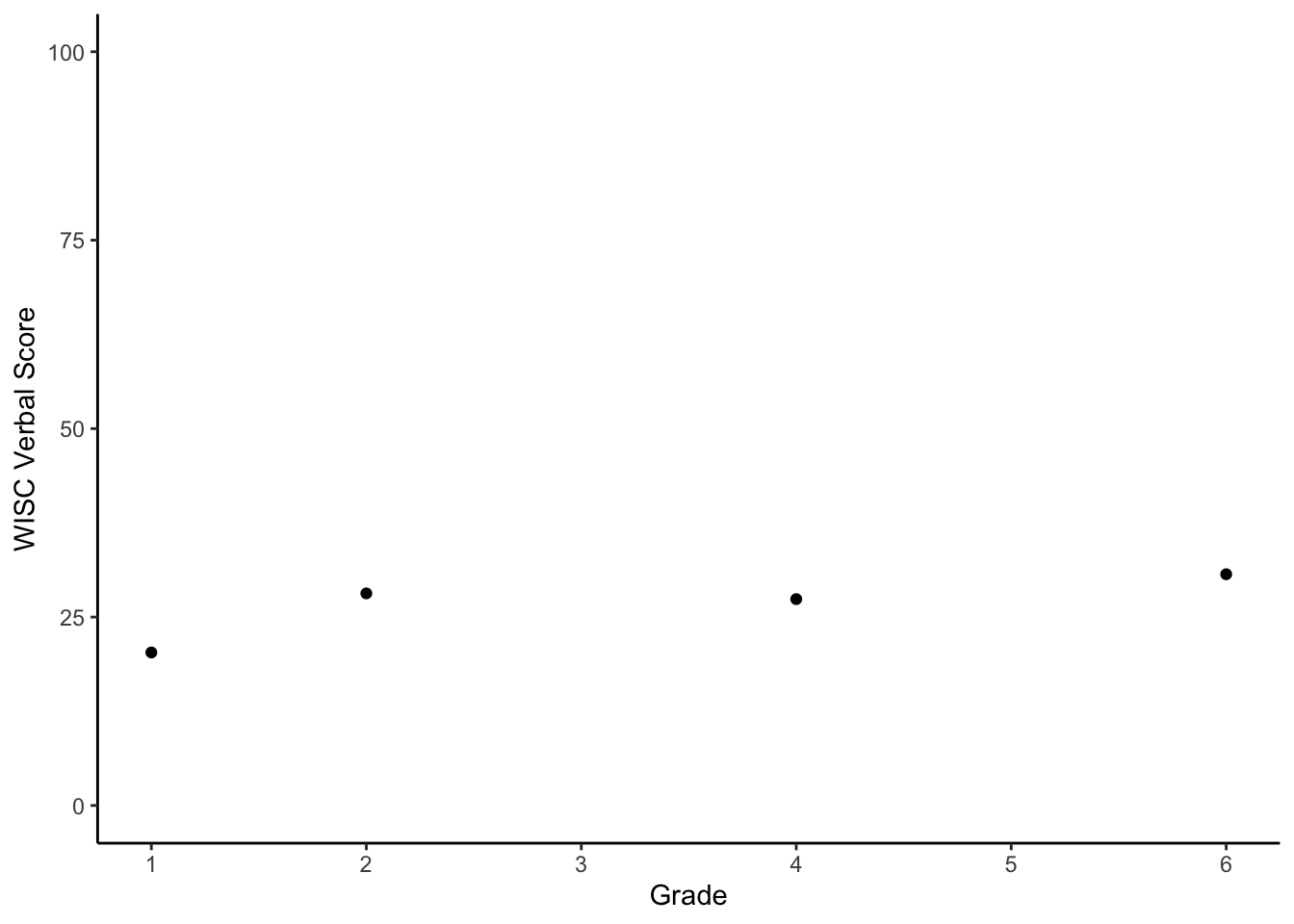

We could connect the dots to see time-adjacent changes.

ggplot(data = verb_id23, aes(x = grade, y = verb, group = id)) +
  geom_point() + 
  geom_line() +
  xlab("Grade") + 
  ylab("WISC Verbal Score") + ylim(0,100) +
  scale_x_continuous(breaks=seq(1,6,by=1)) +
  theme_classic()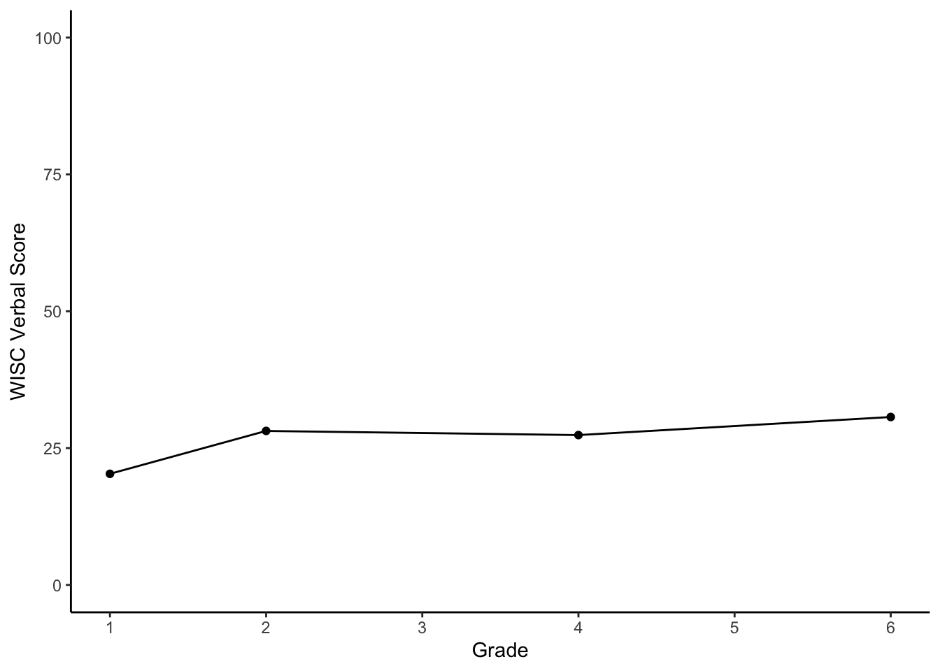

We could also smooth over the repeated measuring using a line of best fit for this individual.

ggplot(data = verb_id23, aes(x = grade, y = verb, group = id)) +
  geom_point() + 
  geom_line() +
  geom_smooth(method=lm, se=FALSE,colour="red", size=1) +
  xlab("Grade") + 
  ylab("WISC Verbal Score") + ylim(0,100) +
  scale_x_continuous(breaks=seq(1,6,by=1)) +
  theme_classic()

## `geom_smooth()` using formula = 'y ~ x'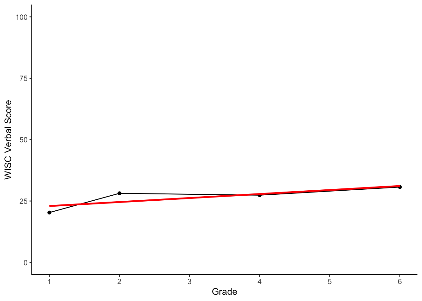

Notice, we can summarize this line with two pieces of information, (1) an intercept, and (2) a slope, each unique to individual 23.

13.3.2 Multiple Individuals

Let’s do an individual regression with time as a predictor. Conceptually, this is a model of intraindividual change corresponding to the plot above.

#regress verb on grade 
linear_id23 <- lm(formula = verb ~ 1 + grade, data = verb_id23, na.action=na.exclude)
#show results
summary(linear_id23) 

## 
## Call:
## lm(formula = verb ~ 1 + grade, data = verb_id23, na.action = na.exclude)
## 
## Residuals:
##    23.1    23.2    23.4    23.6 
## -2.6556  3.5536 -0.4681 -0.4298 
## 
## Coefficients:
##             Estimate Std. Error t value Pr(>|t|)  
## (Intercept)  21.3247     3.1147   6.846   0.0207 *
## grade         1.6308     0.8251   1.977   0.1867  
## ---
## Signif. codes:  0 '***' 0.001 '**' 0.01 '*' 0.05 '.' 0.1 ' ' 1
## 
## Residual standard error: 3.169 on 2 degrees of freedom
## Multiple R-squared:  0.6614, Adjusted R-squared:  0.4921 
## F-statistic: 3.907 on 1 and 2 DF,  p-value: 0.1867

Let’s save the 3 parameters into objects and look at them.

id23_reg_linear <- as.list(coef(linear_id23))
id23_reg_linear

## $`(Intercept)`
## [1] 21.32475
## 
## $grade
## [1] 1.630847

Now let’s do the same thing for all the persons.

We do this in a speedy way using the data.table package.

#converting to a data.table object
verblong_dt <- data.table(verblong)

#collecting regression output by id 
indiv_reg <- verblong_dt[,c(
  reg_1 = as.list(coef(lm(verb ~ grade)))
),by=id]

Let’s look at the moments of the parameters

#converting back to data.frame 
names(indiv_reg)

## [1] "id"                "reg_1.(Intercept)" "reg_1.grade"

indiv_reg_data <- as.data.frame(indiv_reg)

#descriptives
describe(indiv_reg_data[-1])

##                   vars   n  mean   sd median trimmed  mad  min   max range
## reg_1.(Intercept)    1 204 15.15 5.27  15.14   15.23 5.12 0.50 29.41 28.91
## reg_1.grade          2 204  4.67 1.55   4.60    4.61 1.53 1.41  9.38  7.97
##                    skew kurtosis   se
## reg_1.(Intercept) -0.08     0.06 0.37
## reg_1.grade        0.38     0.02 0.11

#correlations among parameters
cor(indiv_reg_data[-1], use="complete.obs",method="pearson")

##                   reg_1.(Intercept) reg_1.grade
## reg_1.(Intercept)         1.0000000  -0.1551763
## reg_1.grade              -0.1551763   1.0000000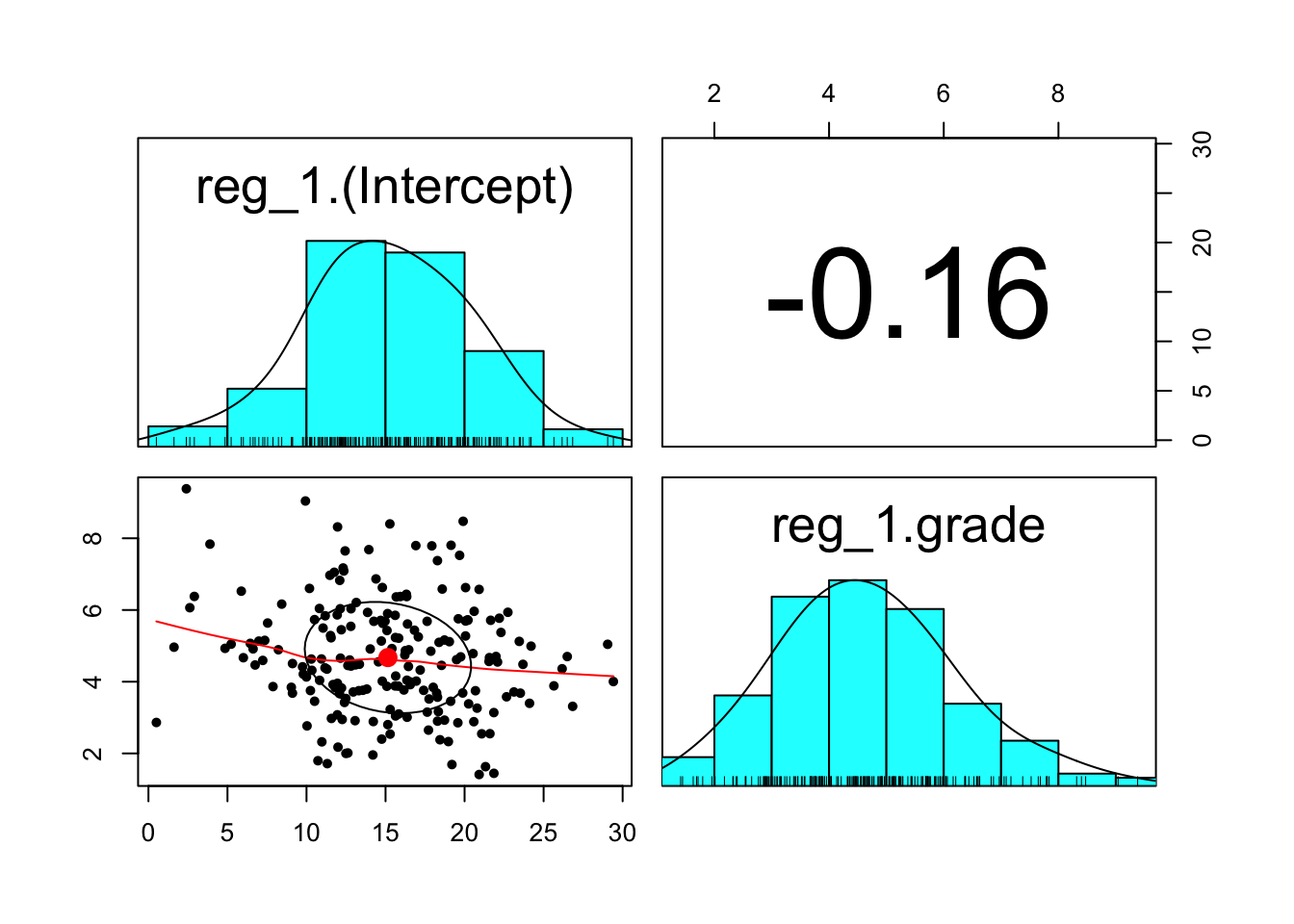

#pairs in the psych library
pairs.panels(indiv_reg_data[-1])

Here, each person has 2 scores (intercept + slope) from the individual-level regression models. Now, let’s plot some of the individual regressions

#making intraindividual change plot
ggplot(data = verblong[which(verblong$id < 30),], aes(x = grade, y = verb, group = id)) +
  geom_smooth(method=lm,se=FALSE,colour="red", size=1) +
  xlab("Grade") + 
  ylab("WISC Verbal Score") + ylim(0,100) +
  scale_x_continuous(breaks=seq(1,6,by=1)) +
  theme_classic()

## `geom_smooth()` using formula = 'y ~ x'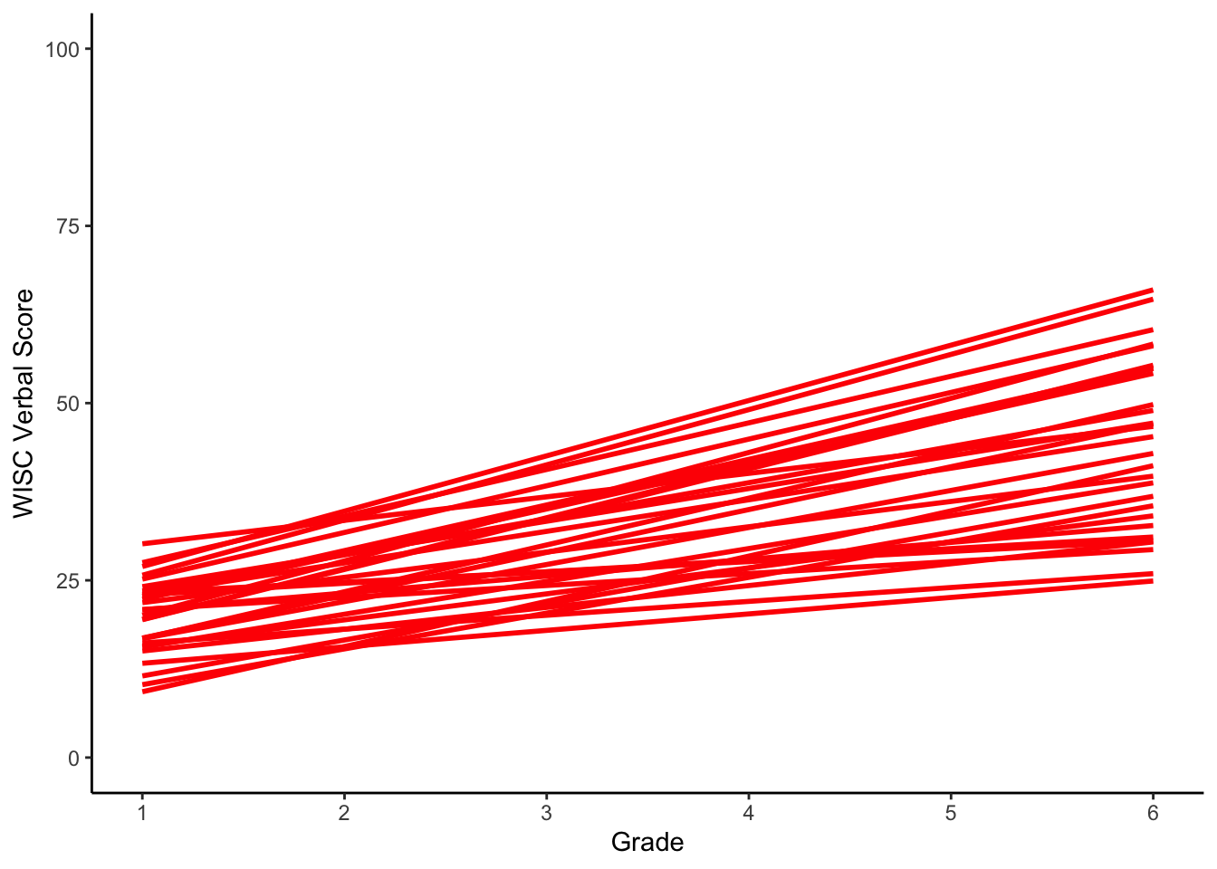

The characteristics of the latent trajectories are captured in two ways:

1. Trajectory Means:

• The average value of the parameters governing the growth trajectory, pooled over the all individuals in the sample. This is the mean starting point and mean rate of change for the sample. These are often called fixed effects.

2. Trajectory Variances:

• The variability of individual cases around the mean trajectory parameters. This is the individual variability in starting point and rate of change over time. Larger variances reflect larger variability in growth. These are often called random effects.

To recap, means captures overall values of parameters that define growth. Variances capture individual variability in those parameters.

Let’s move to our more familiar framework for handling the analysis of “collections” of regressions.