16.4 Hierarchical Clustering
Hierarchical clustering proceeds via an extremely simple algorithm:
Begin by defining some sort of dissimilarity measure between each pair of observations (e.g., Euclidean distance).
Algorithm proceeds iteratively:
- Each of the \(n\) observations is treated as its own cluster
- The two clusters that are most similar are then fused so that there now are \(n-1\) clusters
- Repeat Step 2 until all of the observations belong to one single cluster
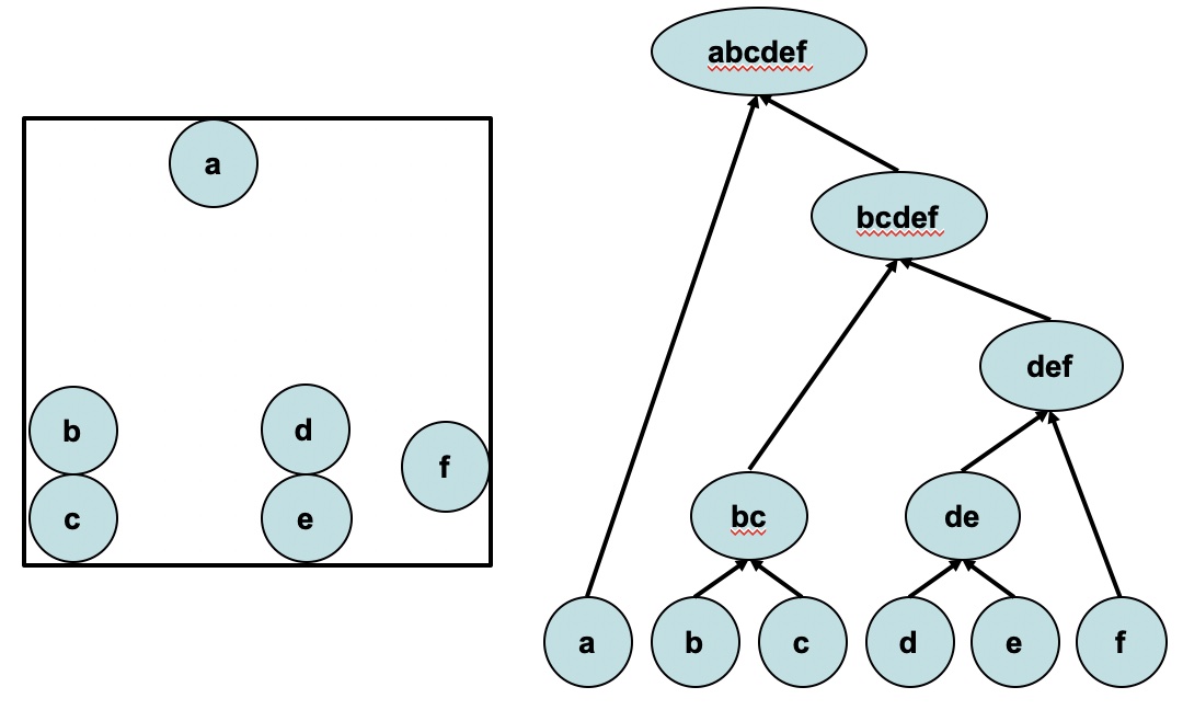
Note this produces not one clustering, but a family of clustering represented by a dendrogram.
16.4.1 Distances
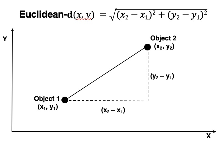
Euclidean distance is a common distance measure. For two dimensions, it is equal to the sum of squares of difference on \(x\) plus the sum of squares of difference on \(y\). Note, variables can differ in scale so it is important to standardize our inputs.
There are many distance measures.
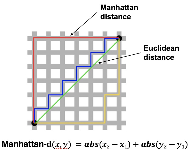 A taxicab geometry is a form of geometry in which the usual distance function or metric of Euclidean geometry is replaced by a new metric in which the distance between two points is the sum of the absolute differences of their Cartesian coordinates.
Taxicab geometry versus Euclidean distance: In taxicab geometry, the red, yellow, and blue paths all have the same shortest path length of 12.
16.4.2 Distance Between Clusters
The concept of dissimilarity between a pair of observations needs to be extended to a pair of groups of observations – what’s the distance between clusters?
This extension is achieved by developing the notion of linkage, which defines the dissimilarity between two groups of observations. Four most common types of linkage: complete, average, single, and centroid. An important fifth is the Ward-method.
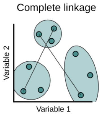
Complete: Maximal intercluster dissimilarity. Compute all pairwise dissimilarities between the observations in cluster A and the observations in cluster B, and record the largest of these dissimilarities. This is sometimes referred to as farthest neighbor clustering.
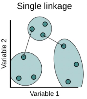
Single: Minimal intercluster dissimilarity. Compute all pairwise dissimilarities between the observations in cluster A and the observations in cluster B, and record the smallest of these dissimilarities.
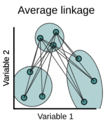
Average: Mean intercluster dissimilarity. Compute all pairwise dissimilarities between the observations in cluster A and the observations in cluster B, and record the average of these dissimilarities.
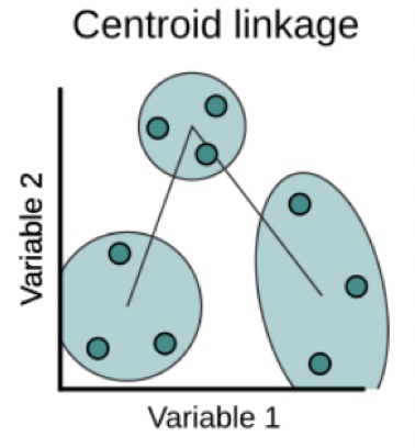
Centroid: Dissimilarity between the centroid for cluster A (a mean vector of length p) and the centroid for cluster B.
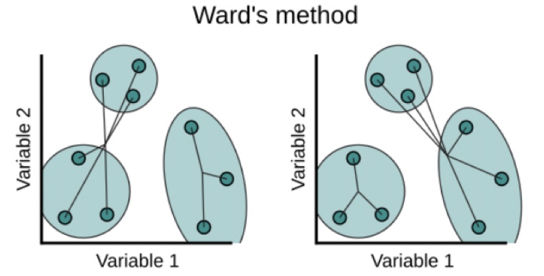
Ward’s Method: minimize within cluster sum of squares. The linkage function specifying the distance between two clusters is computed as the increase in the error sum of squares after fusing two clusters into a single cluster.
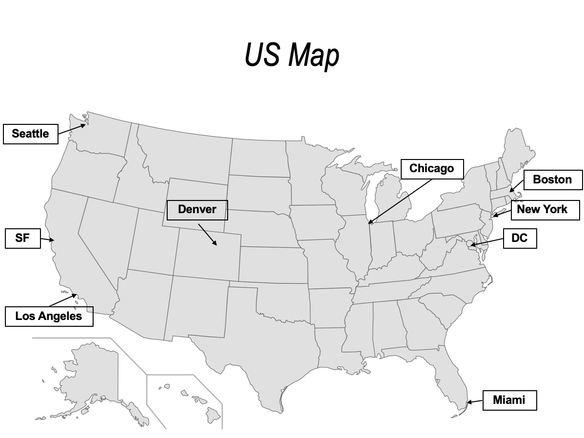
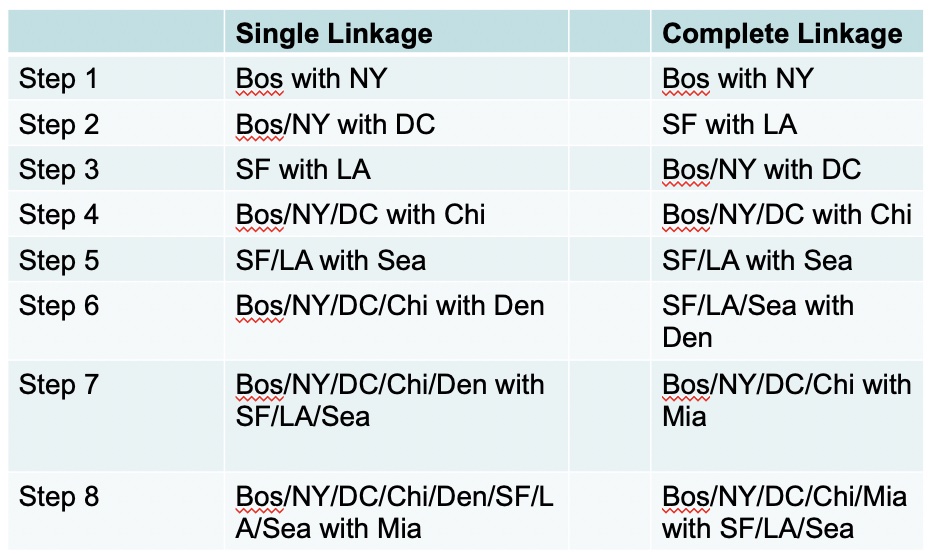
16.4.3 Linkages Applied Example
Let’s take a look at different linkages using this US cities example. First we can calculate the difference among the different cities
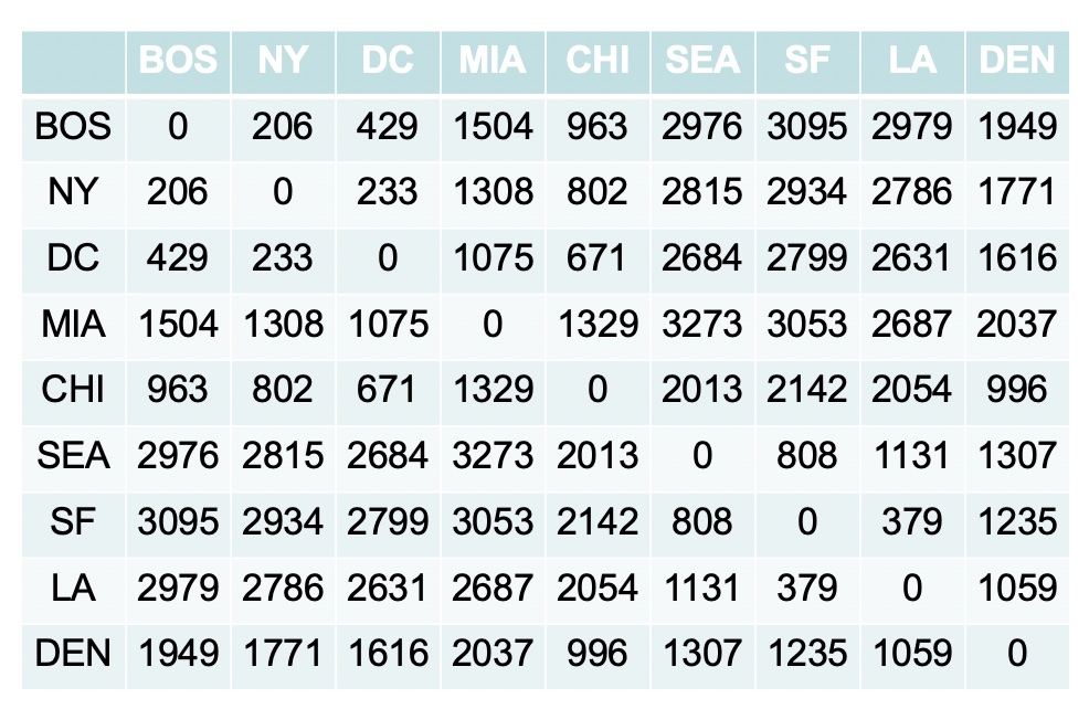
Now, let’s start by making a cluster of Boston and New York.
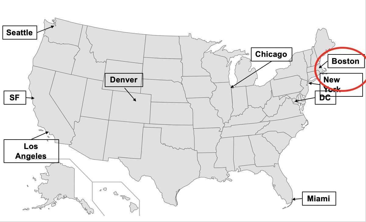
Now compute new dissimilarity matrix. New matrix depends on the linkage approach.
- Complete linkage would use distance from Boston to all other cities because Boston is further than NY
- Single linkage would use distance from NY to all other cities because NY is closer than Boston
- Average linkage would use the mean of the distances from NY and Boston
- Centroid linkage would place a new city half way between NY and Boston and calculate differences from this new city
16.4.4 Dendograms
Now let’s look at the dendograms.
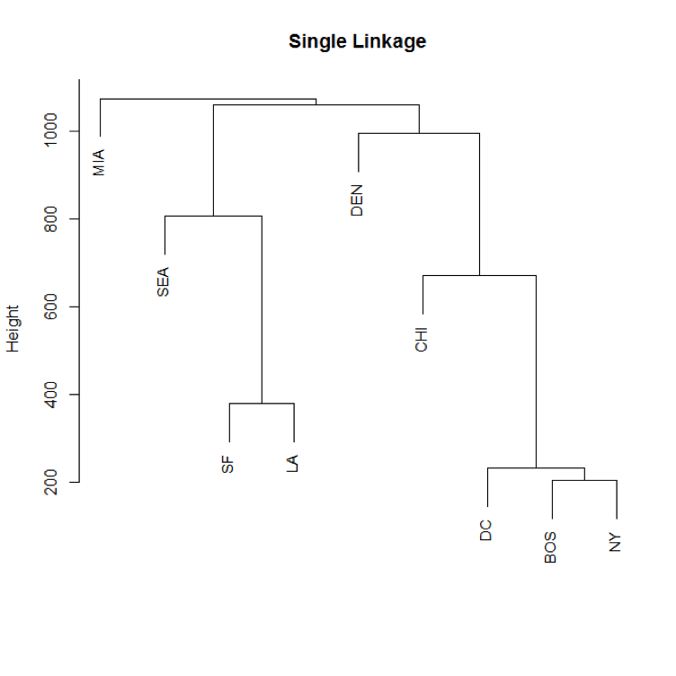
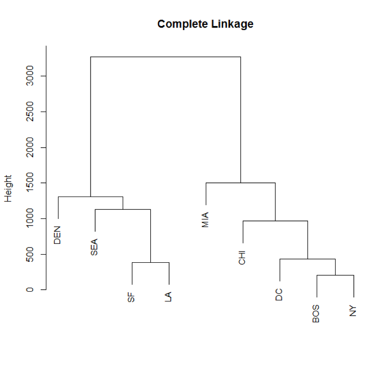 Which one gives us a better solution for the underlying typology?
16.4.4.1 Interpreting Dendograms
- Each leaf of the dendrogram represents one of the \(n\) observations
- Moving up the tree, leaves begin to fuse into branches corresponding to observations that are similar to each other
- Moving higher up, branches fuse, either with leaves or other branches
- The height of the fusion, as measured on the vertical axis, indicates how different the two observations are
- Observations that fuse at the very bottom of the tree are quite similar to each other
- Observations that fuse close to the top of the tree will tend to be quite different
We can draw conclusions about the similarity of two observations based on the location on the vertical axis where branches containing those two observations first are fused.
Generally we are looking for a level above which the lines are long (between-group heterogeneity) and below which the leaves are close (within-group homogeneity).
16.4.4.2 Identifying Clusters in Dendograms
- Make a horizontal cut across the dendrogram
- The distinct sets of observations beneath the cut can be interpreted as clusters
- Therefore, a dendrogram can be used to obtain any number of clusters
Researchers often look at the dendrogram and select by eye a sensible number of clusters based on the heights of the fusion and the number of clusters desired.
The choice of where to cut the dendrogram is not always clear.
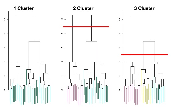
What should we do with this data? 1 2 or 3 groups? You as a researcher have to decide.
Discussion Questions
- Identify a dimension or process central to your own research where you think there is a substantial between-person heterogeneity.
- Identify a set of variables that might be used to classify individuals into meaningful groups as a means to address this heterogeneity.
- With groups or clusters identified how might you empirically assess these groupings?