14.4 Linear Growth (Cortisol)
Now lets fit the series of growth models to the Cortisol data starting with the linear growth model.
14.4.1 Equation
We can write the linear growth model equation as
\[\begin{align} y_{ti} = & \beta_{0i} + \beta_{1i}\text{time}_{1} + e_{ti}, & e_{ti} \sim \mathcal{N}(0,\sigma^{2}_{e}) && \: [\text{Level 1}] \\ \beta_{0i} = & \gamma_{00} + u_{0i}, & u_{0i} \sim \mathcal{N}(0,\sigma^{2}_{u0}) && \: [\text{Level 2}] \\ \beta_{1i} = & \gamma_{10} + u_{1i}, & u_{1i} \sim \mathcal{N}(0,\sigma^{2}_{u1}) && \: \\ y_{ti} = & \underbrace{\gamma_{00} + \gamma_{10}\text{time}_{1}}_{fixed} + \underbrace{u_{0i} + u_{1i}\text{time}_{1}}_{random} + e_{ti}, & && \: [\text{Combined}] \end{align}\]
where
\[\begin{align} \text{time}_{1} = & \{0/8, 1/8, 2/8, 3/8, 4/8, 5/8, 6/8, 7/8, 8/8\}\\ = & \{0.000, 0.125, 0.250, 0.375, 0.500, 0.625, 0.750, 0.875, 1.000\} \end{align}\]
and
- \(y_{ti}\) is the cortisol level for individual \(i\) at time \(t\)
- \(\beta_{0i}\) is the expected baseline level of cortisol for individual \(i\)
- \(\beta_{1i}\) is the expected total change in cortisol for individual \(i\)
- look at coding of time here
- \(\text{time}\) represents the measurement occasion
- \(c_{1}\) has been set to 0
- \(c_{2}\) has been set to 8
- \(e_{it}\) is the time-specific residual score
- \(\gamma_{00}\) is the sample-level mean for the intercept
- \(\gamma_{10}\) is the sample-level mean for the slope
- \(u_{0i}\) is individual \(i\)’s deviation from the sample-level mean of the intercept
- \(u_{1i}\) is individual \(i\)’s deviation from the sample-level mean of the slope
14.4.2 Fit Model
# #linear model
# cort_linear <- lme(cort ~ 1 + timescaled,
#                    random = ~ 1 + timescaled | id,
#                     data = cortisol_long,
#                     na.action = "na.exclude")
# #convergence issues
#
# cort_linear2 <- lmer(cort ~ 1 + timescaled + (1 + timescaled | id),
#                     data = cortisol_long,
#                     na.action = "na.exclude")
# #convergence issues

# cort_linear <- nlme(
#   cort ~ (gamma_00 + u_0i) + (gamma_10 + u_1i)*timescaled,
#   fixed = gamma_00 + gamma_10~1,
#   random = u_0i + u_1i~1,
#   group = ~id,
#   start = c(gamma_00 = 5, gamma_10=1),
#   data = cortisol_long,
#   na.action = "na.exclude",
#   control = lmeControl(maxIter = 1e8, msMaxIter = 1e8)
# )
#
# summary(cort_linear)
# VarCorr(cort_linear)

cort_linear <- nlme(
  cort ~ (gamma_00) + (gamma_10)*timescaled,
  fixed = gamma_00 + gamma_10~1,
  random = gamma_00 + gamma_10~1,
  group = ~id,
  start = c(gamma_00 = 5, gamma_10=1),
  data = cortisol_long,
  na.action = "na.exclude",
  control = lmeControl(maxIter = 1e8, msMaxIter = 1e8)
)

summary(cort_linear)
## Nonlinear mixed-effects model fit by maximum likelihood
## Model: cort ~ (gamma_00) + (gamma_10) * timescaled
## Data: cortisol_long
## AIC BIC logLik
## 1837.972 1860.313 -912.9859
##
## Random effects:
## Formula: list(gamma_00 ~ 1, gamma_10 ~ 1)
## Level: id
## Structure: General positive-definite, Log-Cholesky parametrization
## StdDev Corr
## gamma_00 0.2031304 gmm_00
## gamma_10 4.4907842 1
## Residual 4.3824272
##
## Fixed effects: gamma_00 + gamma_10 ~ 1
## Value Std.Error DF t-value p-value
## gamma_00 8.000588 0.4647815 271 17.213656 0
## gamma_10 10.881176 1.0970635 271 9.918456 0
## Correlation:
## gmm_00
## gamma_10 -0.542
##
## Standardized Within-Group Residuals:
## Min Q1 Med Q3 Max
## -1.8427517 -0.7510168 -0.1820352 0.5969137 2.9508034
##
## Number of Observations: 306
## Number of Groups: 34## id = pdLogChol(list(gamma_00 ~ 1,gamma_10 ~ 1))
## Variance StdDev Corr
## gamma_00 0.04126194 0.2031304 gmm_00
## gamma_10 20.16714270 4.4907842 1
## Residual 19.20566833 4.382427214.4.3 Predicted Trajectories
#obtaining predicted scores for individuals
cortisol_long$pred_linear <- predict(cort_linear)
#obtaining predicted scores for prototype
cortisol_long$proto_linear <- predict(cort_linear, level=0)

# plotting predicted trajectories
# intraindividual change trajetories
ggplot(data = cortisol_long, aes(x = time, y = pred_linear, group = id)) +
  #geom_point(color="black") +
  geom_line(color="black") +
  geom_line(aes(x = time, y = proto_linear), color="red",size=2) +
  xlab("Time") +
  ylab("Cortisol") + ylim(0,30) +
  scale_x_continuous(breaks=seq(0,8,by=1)) +
  theme_classic()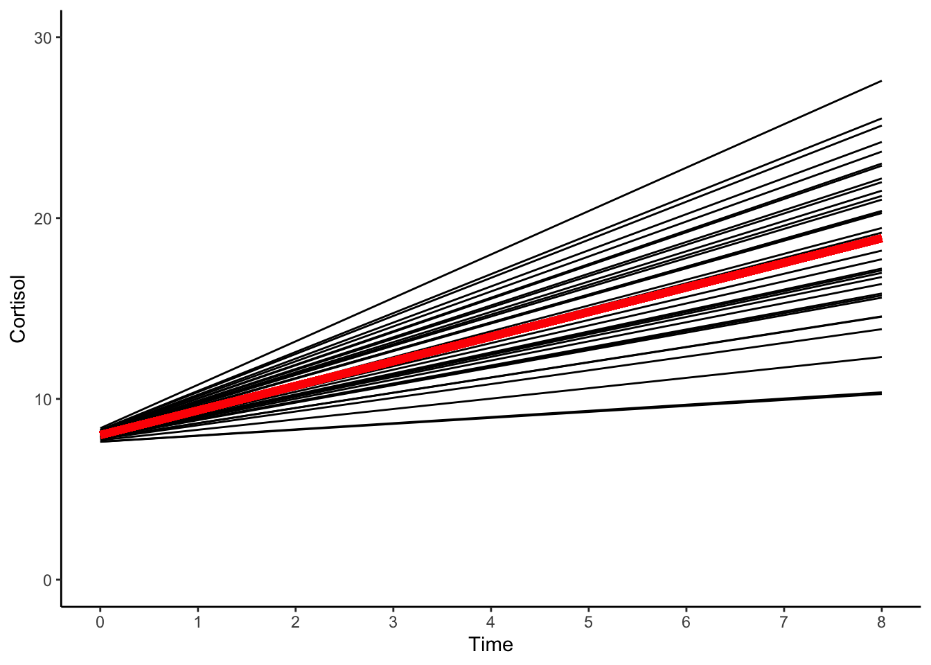
Note that the model has some convergence issues, and the solution has hit a parameter boundary. In this model, and some of the models that follow, the correlation between the random effects in intercept and slope is questionable.
14.4.4 Interpretation
Although we would be reluctant to interpret this model based on the convergence issues. We might say the parameters from the linear model indicate the average person’s baseline level of cortisol is approximately \(8\) mcg/dl and their level of cortisol increases incrementally at each occasion, in total increasing by \(10.9\) units over the course of the remaining eight occasions.
From the plot it appears the linear model fails to capture the intraindividual changes or the interindividual differences in intraindividual change noted in the raw data. It also fails to capture the complexity of the process.