14.5 Quadratic Growth (Cortisol)
The quadratic growth model is a nice first pass at nonlinear modeling. It is a Type I nonlinear method: a linear model that produces nonlinear trajectories.
14.5.1 Equation
The quadratic growth model can be written as
\[\begin{align} y_{ti} = & \beta_{0i} + \beta_{1i}\text{time}_{1}+ \beta_{2i}\text{time}_{2} + e_{ti}, & e_{ti} \sim \mathcal{N}(0,\sigma^{2}_{e}) && \: [\text{Level 1}] \\ \beta_{0i} = & \gamma_{00} + u_{0i}, & u_{0i} \sim \mathcal{N}(0,\sigma^{2}_{u0}) && \: [\text{Level 2}] \\ \beta_{1i} = & \gamma_{10} + u_{1i}, & u_{1i} \sim \mathcal{N}(0,\sigma^{2}_{u1}) && \: \\ \beta_{2i} = & \gamma_{20} + u_{2i}, & u_{2i} \sim \mathcal{N}(0,\sigma^{2}_{u2}) && \: \\ y_{ti} = & \underbrace{\gamma_{00} + \gamma_{10}\text{time}_{1} + \gamma_{20}\text{time}_{2}}_{fixed} + \underbrace{u_{0i} + u_{1i}\text{time}_{1} + u_{2i}\text{time}_{2}}_{random} + e_{ti}, & && \: [\text{Combined}] \end{align}\]
where
\[\begin{align} \text{time}_{1} = \{0.000, 0.125, 0.250, 0.375, 0.500, 0.625, 0.750, 0.875, 1.000\} \text{time}_{2} = \text{time}_{1}^{2} = \{0.000, 0.0157, 0.063, 0.140, 0.250, 0.391, 0.563, 0.766, 1.000\} \end{align}\]
and
- \(y_{ti}\) is the cortisol level for individual \(i\) at time \(t\)
- \(\beta_{0i}\) is the cortisol level at baseline individual \(i\)
- \(\beta_{1i}\) is the expected linear change in cortisol for individual \(i\) at each occasion
- \(\beta_{2i}\) is the expected quadratic change in cortisol for individual \(i\) at each occasion
- \(\text{time}_{1}\) represents the linear change in time
- \(\text{time}_{2}\) represents the quadratic change in time
- \(e_{it}\) is the time-specific residual score (within-person deviation)
- \(\gamma_{00}\) is the fixed effect for the intercept component
- \(\gamma_{10}\) is the fixed effect for the linear component
- \(\gamma_{20}\) is the fixed effect for the quadratic component
- \(u_{0i}\) is individual \(i\)’s deviation from the intercept component
- \(u_{1i}\) is individual \(i\)’s deviation from the linear component
- \(u_{2i}\) is individual \(i\)’s deviation from the quadratic component
14.5.2 Fit Model
#creating the quadratic time variable
cortisol_long$timesq <- cortisol_long$timescaled^2

#quadratic model
# cort_quad <- lme(cort ~ 1 + timescaled + timesq,
#                    random = ~ 1 + timescaled + timesq| id,
#                     data = cortisol_long,
#                     na.action = "na.exclude")
# #convergence issues
#
# cort_quad <- lmer(cort ~ 1 + timescaled + timesq + (1 + timescaled + timesq | id),
#                     data = cortisol_long,
#                     na.action = "na.exclude")
# #convergence issues
# summary(cort_quad)

# cort_quad <- nlme(
#   cort ~ (gamma_00 + u_0i) + (gamma_10 + u_1i)*timescaled + (gamma_20 + u_2i)*timesq,
#   fixed = gamma_00 + gamma_10 + gamma_20 ~1,
#   random = u_0i + u_1i + u_2i ~1,
#   group = ~id,
#   start = c(gamma_00 = 5, gamma_10=1, gamma_20=-1),
#   data = cortisol_long,
#   na.action = "na.exclude",
#   control = lmeControl(maxIter = 1e8, msMaxIter = 1e8)
# )
#
# summary(cort_quad)
# VarCorr(cort_quad)

cort_quad <- nlme(
  cort ~ (gamma_00) + (gamma_10)*timescaled + (gamma_20)*timesq,
  fixed = gamma_00 + gamma_10 + gamma_20 ~1,
  random = gamma_00 + gamma_10 + gamma_20 ~1,
  group = ~id,
  start = c(gamma_00 = 5, gamma_10=1, gamma_20=-1),
  data = cortisol_long,
  na.action = "na.exclude",
  control = lmeControl(maxIter = 1e8, msMaxIter = 1e8)
)

summary(cort_quad)
## Nonlinear mixed-effects model fit by maximum likelihood
## Model: cort ~ (gamma_00) + (gamma_10) * timescaled + (gamma_20) * timesq
## Data: cortisol_long
## AIC BIC logLik
## 1675.114 1712.349 -827.5568
##
## Random effects:
## Formula: list(gamma_00 ~ 1, gamma_10 ~ 1, gamma_20 ~ 1)
## Level: id
## Structure: General positive-definite, Log-Cholesky parametrization
## StdDev Corr
## gamma_00 1.114645 gmm_00 gmm_10
## gamma_10 5.235794 0.632
## gamma_20 5.026802 -0.970 -0.434
## Residual 3.051783
##
## Fixed effects: gamma_00 + gamma_10 + gamma_20 ~ 1
## Value Std.Error DF t-value p-value
## gamma_00 3.60086 0.4686691 270 7.683152 0
## gamma_10 41.05077 2.1882016 270 18.760050 0
## gamma_20 -30.16960 2.1046240 270 -14.334910 0
## Correlation:
## gmm_00 gmm_10
## gamma_10 -0.560
## gamma_20 0.380 -0.872
##
## Standardized Within-Group Residuals:
## Min Q1 Med Q3 Max
## -2.24546377 -0.67200415 0.03095957 0.53189352 2.57525144
##
## Number of Observations: 306
## Number of Groups: 34## id = pdLogChol(list(gamma_00 ~ 1,gamma_10 ~ 1,gamma_20 ~ 1))
## Variance StdDev Corr
## gamma_00 1.242434 1.114645 gmm_00 gmm_10
## gamma_10 27.413535 5.235794 0.632
## gamma_20 25.268739 5.026802 -0.970 -0.434
## Residual 9.313377 3.05178314.5.3 Predicted Trajectories
#obtaining predicted scores for individuals
cortisol_long$pred_quad <- predict(cort_quad)

#obtaining predicted scores for prototype
cortisol_long$proto_quad <- predict(cort_quad, level=0)

#plotting predicted trajectories
#intraindividual change trajetories
ggplot(data = cortisol_long, aes(x = time, y = pred_quad, group = id)) +
  #geom_point(color="black") +
  geom_line(color="black") +
  geom_line(aes(x = time, y = proto_quad), color="red",size=2) +
  xlab("Time") +
  ylab("Cortisol") + ylim(0,30) +
scale_x_continuous(breaks=seq(0,8,by=1)) 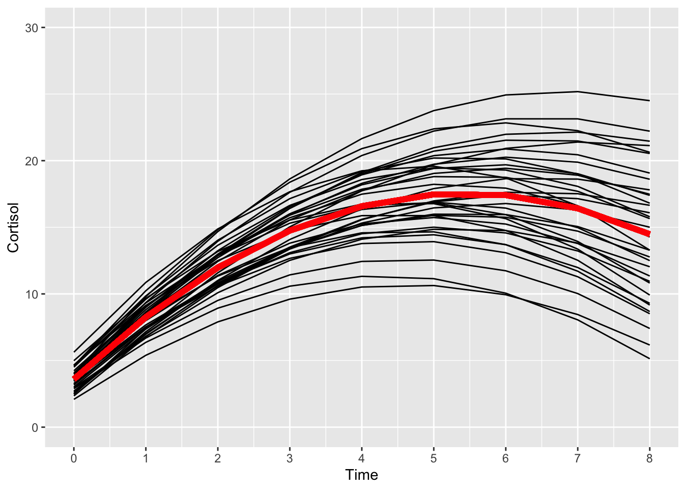
14.5.4 Interpretation
In isolation, the meaning of each parameter in the quadratic growth model is difficult to interpret. The slope parameters must be examined in relation to one another, as it is only their combination that produces a specific trajectory.
For example, consider the mean values of \(\beta_{0}\),\(\beta_{1}\), and \(\beta_{2}\) obtained from the fitted model. The mean of \(\beta_{0} = 3.6\) is interpreted as the average level of cortisol at the baseline assessment (\(t=0\)).
The mean of \(\beta_{1} = 41.1\) could be interpreted as a “gas pedal” of sorts, representing some underlying process that propels cortisol levels higher by the same amount on each successive occasion.
At the same time, the mean of \(\beta_{2} = -30.2\) could be interpreted as representing another underlying process, that of a “brake pedal” that brings cortisol levels lower and that is pressed harder and harder as time moves forward (because \(\beta_{2}\) operates on \(\text{time}_{2}=\text{time}_{1}^{2}\), which consists of squared terms, its influence gains strength on each successive occasion).
From the plot we can see the co-existing “gas pedal” linear process and “brake pedal” quadratic process acting in concert on the individual trajectories. During the first few measurement occasions, when the brake pedal is less influential, cortisol increases, however, during the later occasions, when the brake pedal is stronger, cortisol levels decrease.
Furthermore, \(\beta_{1}\) and \(\beta_{2}\) correlate negatively (\(-.43\)) indicating that when the linear process is strong, the quadratic process is relatively weak.
14.5.5 Interpretational Caution
In closing, quadratic (and most polynomial models) can be difficult to interpret (see Cudeck and du Toit (2002) for more details) in terms of the coefficients alone because
- multiple combination of gas and brake pedals produce similar trajectories
- difficult to understand big versus small gas pedal is without knowing brake pedal
- interindividual differences in these parameters are difficult to map on to particular aspects of an underlying developmental theory of change
- theories are often not so explicit regarding the expected interindividual differences in intraindividual accelerations and deceleration.
14.5.6 Nonlinear or Linear Model?
As we previously mentioned a model is properly termed as nonlinear if the derivatives of the model with respect to the model parameters depend on one or more parameters.
Here is why a polynomial model is not formally a nonlinear model
\[\begin{align} y_{ti} = & \beta_{0i} + \beta_{1i}\text{time}+ \beta_{2i}\text{time}^{2} + e_{ti} \end{align}\]
If we take derivatives of \(y\) with respect to parameters \(\beta_{0i}, \beta_{1i}, \beta_{2i}\) we get
\[\begin{align} \frac{\partial y}{\partial \beta_{0}} = & 1 \\ \frac{\partial y}{\partial \beta_{1}} = & t \\ \frac{\partial y}{\partial \beta_{2}} = & t^2 \\ \end{align}\]
The derivatives do not depend on a model parameter; thus, the polynomial model is linear in its parameters (a linear model that produces a nonlinear trajectory).