14.9 Bilinear Spline (Cortisol)
Spline growth models partition time into discrete periods. Observed changes within each phase can then be described with simple growth models. The discrete segments of the growth model connect at knot points or transition points. Specifically, a bilinear growth model partitions a trajectory into two phases, each defined by a linear trajectory.
Simple spline growth models can be useful for testing specific hypotheses (e.g. does cognitive decline begin at 60 years of age?).
14.9.1 Equation
The equation for the bilinear spline model can be written as
\[\begin{align} y_{ti} = & \beta_{0i} + \beta_{1i}\text{time} + \beta_{2i}\text{max}(\text{time}-k_{1},0)+ e_{ti}, & e_{ti} \sim \mathcal{N}(0,\sigma^{2}_{e}) && \: [\text{Level 1}] \\ \beta_{0i} = & \gamma_{00} + u_{0i}, & u_{0i} \sim \mathcal{N}(0,\sigma^{2}_{u0}) && \: [\text{Level 2}] \\ \beta_{1i} = & \gamma_{10} + u_{1i}, & u_{1i} \sim \mathcal{N}(0,\sigma^{2}_{u1}) && \: \\ \beta_{2i} = & \gamma_{20} + u_{2i}, & u_{2i} \sim \mathcal{N}(0,\sigma^{2}_{u2}) && \: \\ y_{ti} = & \gamma_{00} + \gamma_{10}\text{time} + \gamma_{20}\text{max}(\text{time}-k_{1},0) + u_{0i} + u_{1i}\text{time} + u_{2i}\text{max}(\text{time}-k_{1},0) + e_{ti}, & && \: [\text{Combined}] \end{align}\]
where \[\begin{align} \text{time} = & \{0, 1, 2, 3, 4, 5, 6, 7, 8\} \end{align}\]
and
- \(y_{ti}\) is the repeated measures score for individual \(i\) at time \(t\)
- \(\beta_{0i}\) is the random intercept for individual \(i\) at \(t=0\)
- \(\beta_{1i}\) is the random slope for individual \(i\) when \(t < k\)
- \(\beta_{2i}\) is the change in the random slope for individual \(i\) when \(t > k\)
- rate of change when \(t > k\) is equal to \(\beta_{1i}+\beta_{2i}\)
- \(\text{time}\) represents the time index
- \(k_{1}\) is the knot point (here we set \(k_{1}=4\))
- \(e_{it}\) is the time-specific residual score
- \(\gamma_{00}\) is the fixed-effect for the intercept
- \(\gamma_{10}\) is the fixed-effect for the pre-knot phase
- \(\gamma_{10}\) is the fixed-effect for the post-knot phase
- \(u_{0i}\) is individual \(i\)’s deviation from the intercept fixed effect
- \(u_{1i}\) is individual \(i\)’s deviation from the pre-knot fixed effect
- \(u_{1i}\) is individual \(i\)’s deviation from the post-knot fixed effect
14.9.2 Fit Model
cort_spline <- nlme(
  cort ~ g_00 + g_10*time + g_20*(pmax(time-4,0)),
  data = cortisol_long,
  fixed = g_00 + g_10 + g_20 ~1,
  random = g_00 + g_10 + g_20 ~1,
  groups =~ id,
  start = c(5,4,-5),
  na.action = na.exclude,
  control = lmeControl(maxIter = 1e8, msMaxIter = 1e8)
)

summary(cort_spline)
## Nonlinear mixed-effects model fit by maximum likelihood
## Model: cort ~ g_00 + g_10 * time + g_20 * (pmax(time - 4, 0))
## Data: cortisol_long
## AIC BIC logLik
## 1589.921 1627.157 -784.9606
##
## Random effects:
## Formula: list(g_00 ~ 1, g_10 ~ 1, g_20 ~ 1)
## Level: id
## Structure: General positive-definite, Log-Cholesky parametrization
## StdDev Corr
## g_00 1.8542723 g_00 g_10
## g_10 0.8201397 -0.327
## g_20 1.3000111 0.043 -0.539
## Residual 2.4548968
##
## Fixed effects: g_00 + g_10 + g_20 ~ 1
## Value Std.Error DF t-value p-value
## g_00 3.800588 0.4540068 270 8.371215 0
## g_10 3.722647 0.1856610 270 20.050776 0
## g_20 -4.725000 0.3102078 270 -15.231727 0
## Correlation:
## g_00 g_10
## g_10 -0.560
## g_20 0.312 -0.696
##
## Standardized Within-Group Residuals:
## Min Q1 Med Q3 Max
## -2.29855116 -0.61835284 0.04122658 0.53521318 2.85932981
##
## Number of Observations: 306
## Number of Groups: 34## id = pdLogChol(list(g_00 ~ 1,g_10 ~ 1,g_20 ~ 1))
## Variance StdDev Corr
## g_00 3.4383259 1.8542723 g_00 g_10
## g_10 0.6726292 0.8201397 -0.327
## g_20 1.6900288 1.3000111 0.043 -0.539
## Residual 6.0265184 2.4548968## Approximate 95% confidence intervals
##
## Fixed effects:
## lower est. upper
## g_00 2.911137 3.800588 4.690039
## g_10 3.358916 3.722647 4.086378
## g_20 -5.332732 -4.725000 -4.117268
##
## Random Effects:
## Level: id
## lower est. upper
## sd(g_00) 1.1586971 1.85427234 2.96740711
## sd(g_10) 0.5554807 0.82013974 1.21089562
## sd(g_20) 0.8289480 1.30001108 2.03876347
## cor(g_00,g_10) -0.6962306 -0.32741525 0.17816475
## cor(g_00,g_20) -0.4371323 0.04284905 0.50383364
## cor(g_10,g_20) -0.8071710 -0.53881014 -0.08588567
##
## Within-group standard error:
## lower est. upper
## 2.228902 2.454897 2.70380514.9.3 Predicted Trajectories
Note, this method of plotting can break down with spline models as the plotted trajectories are simply meant to approximate the trajectories of interest. Here they do not connect at the know point, while in the real model they would.
ggplot(data = cortisol_long) +
 geom_line(data=cortisol_long, aes(x = time, y = cort, group=factor(id))) +
 stat_smooth(data=cortisol_long[which(cortisol_long$time<=4),], aes(x=time,y=cort),
             method="lm",colour="#A3A500",size=2) +
 stat_smooth(data=cortisol_long[which(cortisol_long$time>=4),], aes(x=time,y=cort),
             method="lm",colour="#A3A500",size=2) +
  xlab("Timepoint") +
  ylab("Cortisol Level") +
  scale_x_continuous(breaks=seq(0,8,by=10)) +
  scale_y_continuous(breaks = seq(0,50,by=10)) +
  theme_classic() +
  theme(title=element_text(size=12),
        axis.text=element_text(size=12,colour="black"),
        legend.text=element_text(size=12, colour="black"),
        plot.title = element_text(hjust=.5, size=12))
## `geom_smooth()` using formula = 'y ~ x'
## `geom_smooth()` using formula = 'y ~ x'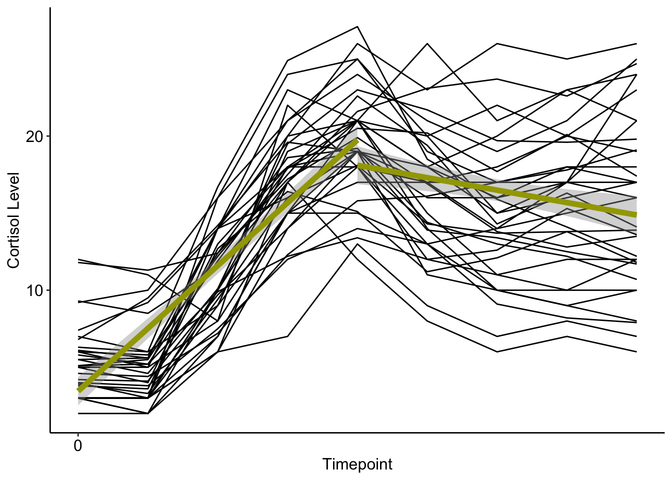
14.9.4 Interpretation
The mean of the random intercept was \(3.8\) mg/dl, indicating the predicted average cortisol at baseline.
The mean of the preknot slope was \(3.7\), indicating the rate of cortisol growht during the baseline and experimental phases.
The mean postknot slope was \(-4.7\), indicating the rate of change decreased by \(4.7\) after timepoint 4.
The variances of the random coefficients were all significant, indicating that subjects varied in each aspect of the growth model.
14.9.4.1 Additional Parameterization
We can also obtain a measure of the post-knot slope directly by reparameterizing our model in the following manner:
\[\begin{align} y_{ti} = & \beta_{0i} + \beta_{1i}\text{min}(\text{time}-k_{1},0) + \beta_{2i}\text{max}(\text{time}-k_{1},0)+ e_{ti}, & e_{ti} \sim \mathcal{N}(0,\sigma^{2}_{e}) && \: [\text{Level 1}] \\ \beta_{0i} = & \gamma_{00} + u_{0i}, & u_{0i} \sim \mathcal{N}(0,\sigma^{2}_{u0}) && \: [\text{Level 2}] \\ \beta_{1i} = & \gamma_{10} + u_{1i}, & u_{1i} \sim \mathcal{N}(0,\sigma^{2}_{u1}) && \: \\ \beta_{2i} = & \gamma_{20} + u_{2i}, & u_{2i} \sim \mathcal{N}(0,\sigma^{2}_{u2}) && \: \\ y_{ti} = & \gamma_{00} + \gamma_{10}\text{min}(\text{time}-k_{1},0) + \gamma_{20}\text{max}(\text{time}-k_{1},0) + u_{0i} + u_{1i}\text{min}(\text{time}-k_{1},0) + u_{2i}\text{max}(\text{time}-k_{1},0) + e_{ti}, & && \: [\text{Combined}] \end{align}\]
where \[\begin{align} \text{time} = & \{0, 1, 2, 3, 4, 5, 6, 7, 8\} \end{align}\]
and
- \(y_{ti}\) is the repeated measures score for individual \(i\) at time \(t\)
- \(\beta_{0i}\) is the random intercept for individual \(i\) at \(t=0\)
- \(\beta_{1i}\) is the random slope for individual \(i\) when \(t < k\)
- \(\beta_{2i}\) is the change in the random slope for individual \(i\) when \(t > k\)
- rate of change when \(t > k\) is equal to \(\beta_{1i}+\beta_{2i}\)
- \(\text{time}\) represents the time index
- \(k_{1}\) is the knot point (here we set \(k_{1}=4\))
- \(e_{it}\) is the time-specific residual score
- \(\gamma_{00}\) is the fixed-effect for the intercept
- \(\gamma_{10}\) is the fixed-effect for the pre-knot phase
- \(\gamma_{10}\) is the fixed-effect for the post-knot phase
- \(u_{0i}\) is individual \(i\)’s deviation from the intercept fixed effect
- \(u_{1i}\) is individual \(i\)’s deviation from the pre-knot fixed effect
- \(u_{1i}\) is individual \(i\)’s deviation from the post-knot fixed effect
14.9.5 Fit Model
cort_spline2 <- nlme(
  cort ~ g_00 + g_10*(pmin(time-4,0)) + g_20*(pmax(time-4,0)),
  data = cortisol_long,
  fixed = g_00 + g_10 + g_20 ~1,
  random = g_00 + g_10 + g_20 ~1,
  groups =~ id,
  start = c(5,5,-5),
  na.action = na.exclude,
  control = lmeControl(maxIter = 1e8, msMaxIter = 1e8)
)

summary(cort_spline2)
## Nonlinear mixed-effects model fit by maximum likelihood
## Model: cort ~ g_00 + g_10 * (pmin(time - 4, 0)) + g_20 * (pmax(time - 4, 0))
## Data: cortisol_long
## AIC BIC logLik
## 1589.921 1627.157 -784.9606
##
## Random effects:
## Formula: list(g_00 ~ 1, g_10 ~ 1, g_20 ~ 1)
## Level: id
## Structure: General positive-definite, Log-Cholesky parametrization
## StdDev Corr
## g_00 3.1964084 g_00 g_10
## g_10 0.8201398 0.836
## g_20 1.1016847 -0.001 0.109
## Residual 2.4548968
##
## Fixed effects: g_00 + g_10 + g_20 ~ 1
## Value Std.Error DF t-value p-value
## g_00 18.691176 0.6165977 270 30.313408 0
## g_10 3.722647 0.1856610 270 20.050775 0
## g_20 -1.002353 0.2248148 270 -4.458572 0
## Correlation:
## g_00 g_10
## g_10 0.792
## g_20 -0.185 -0.134
##
## Standardized Within-Group Residuals:
## Min Q1 Med Q3 Max
## -2.29855112 -0.61835284 0.04122662 0.53521318 2.85932982
##
## Number of Observations: 306
## Number of Groups: 34## id = pdLogChol(list(g_00 ~ 1,g_10 ~ 1,g_20 ~ 1))
## Variance StdDev Corr
## g_00 10.2170269 3.1964084 g_00 g_10
## g_10 0.6726293 0.8201398 0.836
## g_20 1.2137092 1.1016847 -0.001 0.109
## Residual 6.0265184 2.4548968