5.8 The Linear Probability Model
While we are discussing the assumptions of OLS it is worth pausing to consider a model for dichotomous outcomes: the linear probability model (LPM).
In the LPM we don’t do anything fancy with a binary outcome variable. Instead, we simply apply OLS as we would with a continuous out come variable. Since we aren’t considering the normality of our outcome you might be curious how our assumptions would hold.
Remembering the assumptions of OLS:
- \(\mathbb{E}(\epsilon_{i}) = 0\)
- \(\mathbb{E}(\epsilon_{i}^2) = \sigma^2\) for all \(i\) (homoscedasticity)
- \(\mathbb{E}(\epsilon_{i}\epsilon_{j}) = 0\) for all \(i \neq j\)
- No perfect collinearity among \(x\) variables
- \(\mathbb{C}(\epsilon_{i},x_{qi}) = 0\) for all \(i\) and \(k\)
Which assumptions are needed for consistency and asymptotic unbiasedness?
- No perfect collinearity among \(x\) variables
- Errors uncorrelated with all \(x\) variables.
In regard to (4) having a dependent variable valued at \(0,1\) does not cause any problems. In regard to (5), again no, nothing about a dichotomous outcome violates this assumption.
Therefore, in this model \(\mathbf{\hat\beta}\) is still consistent and asymptotically unbiased.
What about the remaining assumptions?
- Homoscedasticity
Here, a dichotomous outcome does inherently violate the assumption of homoskedasticity.
Why is this case? It can be shown that \(\mathbb{V}(\epsilon_{i})\) now directly depends on the value of \(x\) that is taken. If the \(ith\) person has one set of values for the \(x\) variables, and another individual \(j\) has another set, the estimates of \(\mathbb{V}(\epsilon_{i})\) and \(\mathbb{V}(\epsilon_{j})\) will differ. This can be seem by looking at the variance of a Bernoulli random variable.
This means estimate of variance of \(\mathbf{\hat\beta}\) is no longer reliable, SEs and significance tests possibly inaccurate. However, this could be addressed using robust standard errors.
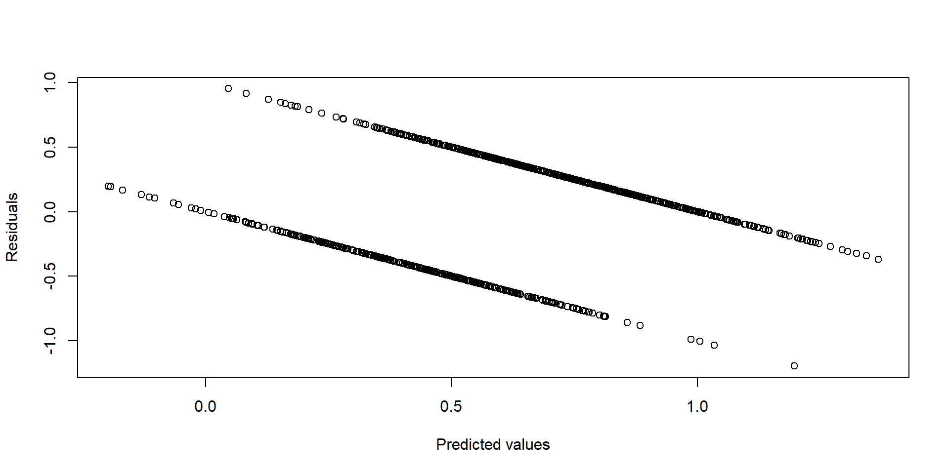
It is common to look at plots of predicted values vs residuals to diagnose heteroskedasticity. Generally one would like to see a random blob of points without any discernible pattern. Here is an example of what that plot might look like for an LPM model. Each line represents a different outcome, \(y=0\), or \(y=1\).