14.7 Exponential Growth (Cortisol)
Now let’s consider a model that is nonlinear in the parameters (Type II), the exponential growth model. This is a nonlinear model that also produces a nonlinear trajectory.
\[\begin{align} y_{ti} = & \beta_{0i} + \beta_{1i}(1-e^{-\alpha\text{time}}) + e_{ti}, & e_{ti} \sim \mathcal{N}(0,\sigma^{2}_{e}) && \: [\text{Level 1}] \\ \beta_{0i} = & \gamma_{00} + u_{0i}, & u_{0i} \sim \mathcal{N}(0,\sigma^{2}_{u0}) && \: [\text{Level 2}] \\ \beta_{1i} = & \gamma_{10} + u_{1i}, & u_{1i} \sim \mathcal{N}(0,\sigma^{2}_{u1}) && \: \\ y_{ti} = & \gamma_{00} + \gamma_{10}\text{time} + u_{0i} + u_{1i}\text{time} + e_{ti}, & && \: [\text{Combined}] \end{align}\]
where
\[\begin{align} \text{time} = & \{0/8, 1/8, 2/8, 3/8, 4/8, 5/8, 6/8, 7/8, 8/8\}\\ = & \{0.000, 0.125, 0.250, 0.375, 0.500, 0.625, 0.750, 0.875, 1.000\} \end{align}\]
and
- \(y_{ti}\) is the repeated measures score for individual \(i\) at time \(t\)
- \(\beta_{0i}\) is the random intercept for individual \(i\)
- individual \(i\)’s asymptotic level or the limit of individual capacity for cortisol
- note in this model, the intercept represents individual performance toward the end of observation period
- \(\beta_{1i}\) is the amount of change from the intercept to the asymptotic level for individual \(i\)
- \(\beta_{1i}\) represents an individual’s potential for change from his or her initial level
- \(\beta_{0i}+\beta_{1i}\) represents the baseline level for individual \(i\)
- \(\alpha\) is an estimated parameter that represents the rate of approach to the asymptotic level
- \(\text{time}\) represents the measurement occasion
- \(e_{it}\) is the time-specific residual score
- \(\gamma_{00}\) is the fixed-effect for the intercept
- \(\gamma_{10}\) is the fixed-effect for the rate of change
- \(u_{0i}\) is individual \(i\)’s deviation from the intercept fixed effect
- \(u_{1i}\) is individual \(i\)’s deviation from the shape fixed effect
14.7.1 Fit Model
# cort_expo <- nlme(
#   cort ~ (gamma_00 + u_0i) + (gamma_10 + u_1i)*(exp(-1*alpha*timescaled)),
#   fixed = gamma_00 + gamma_10 + alpha ~1,
#   random = u_0i + u_1i~1,
#   group = ~id,
#   start = c(gamma_00=17, gamma_10=-14, alpha=0.5),
#   data = cortisol_long,
#   na.action = "na.exclude",
#   control = lmeControl(maxIter = 1e8, msMaxIter = 1e8)
# )
#
# summary(cort_expo)
# VarCorr(cort_expo)

cort_expo <- nlme(
  cort ~ (gamma_00) + (gamma_10)*(exp(-1*alpha*timescaled)),
  fixed = gamma_00 + gamma_10 + alpha ~1,
  random = gamma_00 + gamma_10~1,
  group = ~id,
  start = c(gamma_00=17, gamma_10=-14, alpha=0.5),
  data = cortisol_long,
  na.action = "na.exclude",
  control = lmeControl(maxIter = 1e8, msMaxIter = 1e8)
)
## Warning in nlme.formula(cort ~ (gamma_00) + (gamma_10) * (exp(-1 * alpha * :
## Iteration 4, LME step: nlminb() did not converge (code = 1). PORT message:
## function evaluation limit reached without convergence (9)## Nonlinear mixed-effects model fit by maximum likelihood
## Model: cort ~ (gamma_00) + (gamma_10) * (exp(-1 * alpha * timescaled))
## Data: cortisol_long
## AIC BIC logLik
## 1730.241 1756.306 -858.1203
##
## Random effects:
## Formula: list(gamma_00 ~ 1, gamma_10 ~ 1)
## Level: id
## Structure: General positive-definite, Log-Cholesky parametrization
## StdDev Corr
## gamma_00 3.671940 gmm_00
## gamma_10 3.984773 -1
## Residual 3.594813
##
## Fixed effects: gamma_00 + gamma_10 + alpha ~ 1
## Value Std.Error DF t-value p-value
## gamma_00 17.202377 0.7688426 270 22.37438 0
## gamma_10 -13.735027 0.9550594 270 -14.38133 0
## alpha 4.110241 0.4853610 270 8.46842 0
## Correlation:
## gmm_00 gmm_10
## gamma_10 -0.788
## alpha -0.442 0.077
##
## Standardized Within-Group Residuals:
## Min Q1 Med Q3 Max
## -2.06791703 -0.69558253 -0.03451498 0.60588520 2.72990814
##
## Number of Observations: 306
## Number of Groups: 34## id = pdLogChol(list(gamma_00 ~ 1,gamma_10 ~ 1))
## Variance StdDev Corr
## gamma_00 13.48314 3.671940 gmm_00
## gamma_10 15.87841 3.984773 -1
## Residual 12.92268 3.59481314.7.2 Predicted Trajectories
#obtaining predicted scores for individuals
cortisol_long$pred_expo <- predict(cort_expo)

#obtaining predicted scores for prototype
cortisol_long$proto_expo <- predict(cort_expo, level=0)


#plotting predicted trajectories
#intraindividual change trajetories
ggplot(data = cortisol_long, aes(x = time, y = pred_expo, group = id)) +
  #geom_point(color="black") +
  geom_line(color="black") +
  geom_line(aes(x = time, y = proto_expo), color="red",size=2) +
  xlab("Time") +
  ylab("Cortisol") + ylim(0,30) +
  scale_x_continuous(breaks=seq(0,8,by=1)) +
  theme_classic()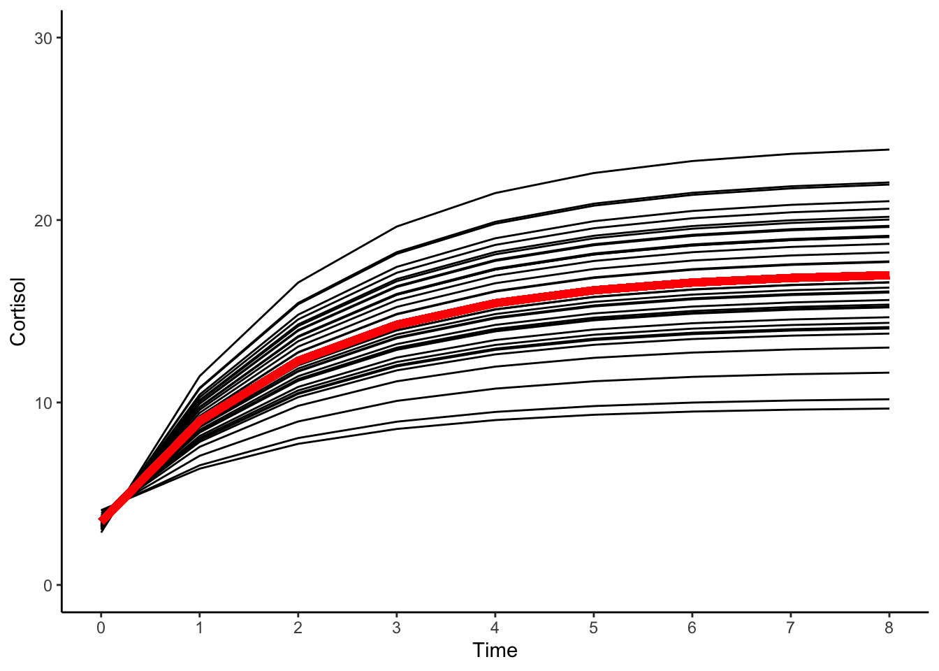
14.7.3 Interpretation
Fitted to our example data, we articulate a theory wherein individuals enter the testing situation at some baseline level of cortisol (which on average is given by mean of \(beta_{0}\), \(17.2\), plus the mean of \(\beta_{1}\), \(-13.7\), which equals \(3.5\)).
After beginning the simulator cortisol levels are driven at the exponential rate of \(\alpha=4.1\) to some personal limit or asymptote (with the average limit being \(17.2\)).
14.7.4 Nonlinear or Linear Model?
What about the exponential model. Here is is why a exponential model is formally a nonlinear model
\[\begin{align} y_{ti} = & \beta_{0i} + \beta_{1i}(1-e^{-\alpha\text{time}}) + e_{ti} \end{align}\]
If we take derivatives of \(y\) with respect to parameters \(\beta_{0i}, \beta_{1i}, \alpha\) we get
\[\begin{align} \frac{\partial y}{\partial \beta_{0}} = & 1 \\ \frac{\partial y}{\partial \beta_{1}} = & (1-e^{-\alpha\text{time}}) \\ \frac{\partial y}{\partial \alpha} = & \beta_{1} \text{time}(1-e^{-\alpha\text{time}}) \end{align}\]
The derivatives depend on non-constant (or estimated coefficients). This model is multiplicative nonlinear it its parameters. A nonlinear model that produces a nonlinear trajectory.