11.9 Example Data II
Now, let us compare the common situation where we have a predictor of interest. Castro-Schilo and Grimm (2018) consider a situation common to behavioral science researchers.
Sofia, a close relationships’ researcher, is interested in examining change in relationship satisfaction before and after marriage. Specifically, she wants to know whether cohabiting prior to marriage has an effect on changes in relationship satisfaction. As she plans her data analysis strategy, Sofia realizes she has two options: (1) use the postmarriage relationship satisfaction score as her outcome and include the premarriage score in her analysis as a predictor, in addition to whether or not couples cohabited prior to marriage to account for individual differences in baseline relationship satisfaction (known as residualized change approach) or (2) compute the difference between the postmarriage relationship satisfaction score and the premarriage relationship satisfaction score and use it as her outcome to test the effect of cohabiting prior to marriage (known as difference score approach). Which of these two strategies is most appropriate? Should both strategies provide the same results? Sofia has heard difference scores have a bad reputation, why is that? Are there additional strategies Sofia is not aware of that might be preferred over her current options?
11.9.1 Generate Some Data According to (Castro-Schilo and Grimm 2018)
Let’s generate some data according to the example from Castro-Schilo and Grimm (2018). Below is one possible data generating model.
We will consider two scenarios. In both scenarios the following facts will be true:
- Both data sets have an equal number of dyads that did and did not cohabit
- Cohabitation had a null effect on changes in relationship satisfaction.
- Dyads did not exhibit any changes in relationship satisfaction over time.
In this first example dataset, however, there are preexisting groups at the premarriage assessment. That is, because in a real investigation of cohabitation a controlled experiment would not be feasible, we generated one data set with lower relationship satisfaction at baseline for dyads who reported cohabiting.
Note that our description of the first dataset corresponds to the assumption made by the difference score model (i.e., no change between groups across time under the assumption of the null hypothesis for the key predictor; there are two populations at baseline).
# set a seed so we all have the same data
set.seed (1234)

# create an id variable (N = 100 in each group)
id <- c(1:100, 1:100)

# create a time variable (0 = time 1, 1 = time 2)
time <- c(rep(0, 100), rep(1, 100))

# create grouping variable with equal number cohabiting (1) and not (0)
cohabit <- rep(c(0,1), 100)

# put all variables in a dataframe
data <- data.frame(id, cohabit, time)

# generate dataset A
data_A <- data
data_A$score <-
  4.5 +                          # intercept
  -2*data_A$cohabit +            # difference in cohabitation
  0*data_A$time +                # effect of time
  0*data_A$cohabit*data_A$time + # interaction
  rnorm(200, 0, 0.3)             # error


# Make into wide format for computing difference score
data_A <- reshape(
  data_A,
  v.names = 'score',
  timevar = "time",
  idvar = "id",
  direction= "wide"
)

# assign appropriate variable names
names(data_A) <- c('id', 'cohabit', 'score1', 'score2')

# compute difference variable
data_A$diff <- data_A$score2 - data_A$score1

# declare cohabiting variable as a factor (categorical variable)
data_A$cohabit <- factor(data_A$cohabit)
11.9.2 Plot Data
# visualize the data
library(ggplot2)
ggplot(data_A, aes(x = score1, y = score2, shape= cohabit)) +
  geom_point(size = 3) +
  geom_smooth(method = lm, se = F) +
  xlab("Relationship Satisfaction Time 1") +
  ylab("Relationship Satisfaction Time 2")
## `geom_smooth()` using formula = 'y ~ x'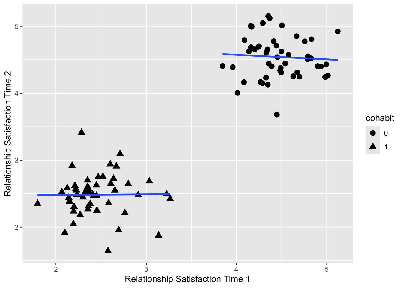
11.9.3 Fit Residualized Change Model
Recall that the main interest in these analyses is to assess the potential effect of cohabitation on changes in relationship satisfaction.
According to the residualized change model we fit to data set A (which is an ANCOVA model in this application because of the categorical predictor), the factors explain 92% of the variance in the outcome and results suggest there is a statistically and practically significant effect of cohabitation in dyad’s relationship satisfaction at Time 2, controlling for baseline relationship satisfaction.
##
## Call:
## lm(formula = score2 ~ score1 + cohabit, data = data_A)
##
## Residuals:
##      Min       1Q   Median       3Q      Max
## -0.86084 -0.17640  0.00684  0.17019  0.92449
##
## Coefficients:
##             Estimate Std. Error t value Pr(>|t|)
## (Intercept)  4.66901    0.46562  10.028  < 2e-16 ***
## score1      -0.02875    0.10390  -0.277    0.783
## cohabit1    -2.11473    0.21860  -9.674 6.78e-16 ***
## ---
## Signif. codes:  0 '***' 0.001 '**' 0.01 '*' 0.05 '.' 0.1 ' ' 1
##
## Residual standard error: 0.3114 on 97 degrees of freedom
## Multiple R-squared:  0.9183, Adjusted R-squared:  0.9167
## F-statistic: 545.4 on 2 and 97 DF,  p-value: < 2.2e-16
11.9.4 Fit Difference Score Model
##
## Call:
## lm(formula = diff ~ cohabit, data = data_A)
##
## Residuals:
##      Min       1Q   Median       3Q      Max
## -1.29920 -0.22982  0.00904  0.28891  1.09081
##
## Coefficients:
##             Estimate Std. Error t value Pr(>|t|)
## (Intercept)  0.07941    0.06212   1.278    0.204
## cohabit1    -0.04002    0.08786  -0.455    0.650
##
## Residual standard error: 0.4393 on 98 degrees of freedom
## Multiple R-squared:  0.002113,   Adjusted R-squared:  -0.00807
## F-statistic: 0.2075 on 1 and 98 DF, p-value: 0.6498##
## Call:
## lm(formula = diff ~ cohabit + score1, data = data_A)
##
## Residuals:
## Min 1Q Median 3Q Max
## -0.86084 -0.17640 0.00684 0.17019 0.92449
##
## Coefficients:
## Estimate Std. Error t value Pr(>|t|)
## (Intercept) 4.6690 0.4656 10.028 < 2e-16 ***
## cohabit1 -2.1147 0.2186 -9.674 6.78e-16 ***
## score1 -1.0287 0.1039 -9.901 < 2e-16 ***
## ---
## Signif. codes: 0 '***' 0.001 '**' 0.01 '*' 0.05 '.' 0.1 ' ' 1
##
## Residual standard error: 0.3114 on 97 degrees of freedom
## Multiple R-squared: 0.5037, Adjusted R-squared: 0.4935
## F-statistic: 49.23 on 2 and 97 DF, p-value: 1.75e-15In contrast, when we fit the difference score model to the same data, less than 1% of the variance in the outcome is explained by the model, and results suggested that cohabitation did not have an effect on relationship satisfaction change. As expected, the inferences from these models are strikingly different, which is an example of Lord’s paradox and can be attributed to the differences in baseline scores across couples who cohabit and those who do not.