14.1 Review of Linear Growth
14.1.1 Theory of Linear Growth
Before diving into nonlinear model let’s briefly review linear growth.
Theory of Intraindividual Change
Individuals’ behavior changes over time at a pre-determined, unchanging (stable) rate. For a linear growth model to hold we need an explanation regarding what is driving the pre-determined rate of change
- A one-time event with a forever lasting effect?, or
- A continuous event with a stable effect?
Theory of Interindividual Differences
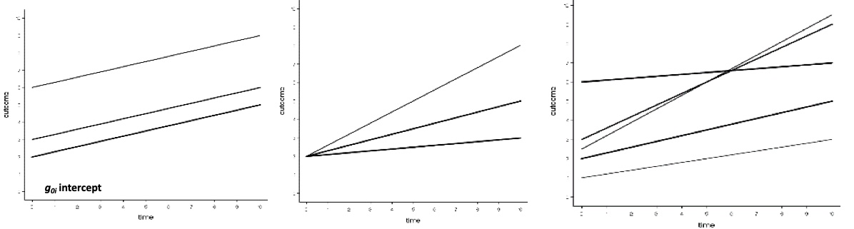
We suppose individuals can differ in their “initial” level of behavior
- Need an explanation of why individuals have different “initial” levels
We suppose individuals differ in their rate of change
- Need an explanation of why individuals have different rates of change
14.1.2 Characteristics of Linear Growth
Benefits of Linear Growth Models
- Simple developmental pattern
- Easily interpretable parameters
- Level: predicted score when \(t = 0\)
- Slope: rate of change in \(y\) for a \(1-unit\) change in \(t\)
Limitations of Linear Growth Models
- Often does not truly match the developmental process theories
- Difficult to generalize outside of observation period
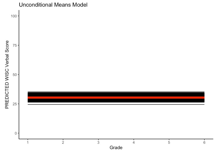
14.1.3 No Growth Model
First, let’s consider the no growth model. Remember, the no growth model suggests individuals differ only in terms of their overall level of a given construct, and this level does not change across time. It is often useful as an initial model to determine whether future analyses are warranted.
14.1.3.2 No Growth Equations
\[\begin{align} y_{ti} = & \beta_{0i} + e_{ti}, & e_{ti} \sim \mathcal{N}(0,\sigma^{2}_{e}) && \: [\text{Level 1 Equation}] \\ \beta_{0i} = & \gamma_{00} + u_{0i}, & u_{0i} \sim \mathcal{N}(0,\sigma^{2}_{u0}) && \: [\text{Level 2 Equation}] \\ y_{ti} = & \underbrace{\gamma_{00}}_{fixed} + \underbrace{u_{0i}}_{random} + e_{ti}, & && \: [\text{Combined Equation}] \end{align}\]
where
- \(y_{ti}\) is the repeated measures score for individual \(i\) at time \(t\)
- \(\beta_{0i}\) is the random intercept for individual \(i\) (person-specific mean)
- \(e_{ti}\) is the time-specific residual score (within-person deviation)
- \(\gamma_{00}\) is the sample mean for the intercept (grand mean)
- \(u_{0i}\) is individual \(i\)’s deviation from the sample mean (between person deviation)
14.1.3.3 No Growth Code
Here, we present code for fitting the no growth model in the nlme package using both compact and detailed model syntax.
um_nlme <- nlme::nlme(
  verb ~ gamma_00 + u_0i,
  data = verblong,
  fixed = gamma_00~1,
  random = u_0i~1,
  group = ~id,
  na.action="na.omit",
  start = c(gamma_00 = mean(verblong$verb))
)
summary(um_nlme)

um_lme <- nlme::lme(
  fixed= verb ~ 1,
  random = ~ 1|id,
  data = verblong,
  na.action = na.exclude
)
summary(um_lme)
14.1.4 Random Intercept Model
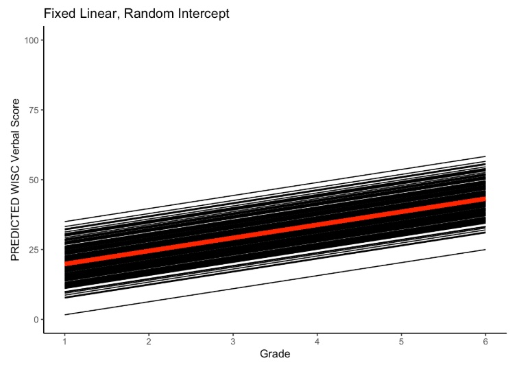
14.1.4.2 Random Intercept Equations
\[\begin{align} y_{ti} = & \beta_{0i} + \beta_{1i}\frac{\text{time}_{}-c_{1}}{c_{2}} + e_{ti}, & e_{ti} \sim \mathcal{N}(0,\sigma^{2}_{e}) && \: [\text{Level 1}] \\ \beta_{0i} = & \gamma_{00} + u_{0i}, & u_{0i} \sim \mathcal{N}(0,\sigma^{2}_{u0}) && \: [\text{Level 2}] \\ \beta_{1i} = & \gamma_{10}, & && \: \\ y_{ti} = & \underbrace{\gamma_{00} + \gamma_{10}\frac{\text{time}-c_{1}}{c_{2}}}_{fixed} + \underbrace{u_{0i}}_{random} + e_{ti}, & && \: [\text{Combined}] \end{align}\]
where
\[\begin{align} u_{0i} \sim \left( \begin{array}{r} 0 \end{array}, \begin{array}{c} \sigma^{2}_{u0} \end{array}\right), \end{align}\]
and
- \(y_{ti}\) is the repeated measures score for individual \(i\) at time \(t\)
- \(\beta_{0i}\) is the random intercept for individual \(i\)
- predicted score for individual \(i\) when \(\text{time}=0\)
- \(\beta_{1i}\) is the sample-level mean for the slope (\(\beta_{1i}=\gamma_{10}\))
- predicted rate of change for individual \(i\) with a 1-unit change in \(\text{time}\)
- \(\text{time}\) represents time and could be grade, age, year, etc.
- predicted rate of change for individual \(i\) with a 1-unit change in \(\text{time}\)
- \(c_{1}\) constant used to center the intercept
- \(c_1\) is often set to \(1\) to center the intercept at the first occasion
- \(c_{2}\) constant chosen to scale the slope
- \(c_2\) is often set to \(1\) to scale the slope in terms of the units of \(\text{time}\)
- \(e_{it}\) is the time-specific residual score (within-person deviation)
- \(\gamma_{00}\) is the sample-level mean for the intercept
- \(\gamma_{10}\) is the sample-level mean for the slope
- \(u_{0i}\) is individual \(i\)’s deviation from the sample-level mean of the intercept
14.1.4.3 Random Intercept Code
Here, we present code for fitting the random intercept model in the nlme package using both compact and detailed model syntax.
ri_nlme <- nlme::nlme(
  verb ~ (gamma_00 + u_0i) + (gamma_10)*grade,
  data = verblong,
  fixed = gamma_00 + gamma_10~1,
  random = u_0i~1,
  group = ~id,
  na.action="na.omit",
  start = c(gamma_00 = 30, gamma_10=10)
)
summary(ri_nlme)

ri_lme <- nlme::lme(
  fixed = verb ~ 1 + grade,
  random = ~ 1|id,
  data=verblong,
  na.action = na.exclude,
  method = "ML"
)
summary(ri_lme)
14.1.5 Linear Growth Model
Now let’s consider the linear growth model
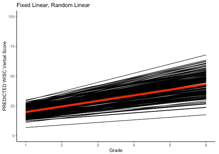
14.1.5.2 Linear Growth Equations
\[\begin{align} y_{ti} = & \beta_{0i} + \beta_{1i}\text{time} + e_{ti}, & e_{ti} \sim \mathcal{N}(0,\sigma^{2}_{e}) && \: [\text{Level 1}] \\ \beta_{0i} = & \gamma_{00} + u_{0i}, & u_{0i} \sim \mathcal{N}(0,\sigma^{2}_{u0}) && \: [\text{Level 2}] \\ \beta_{1i} = & \gamma_{10} + u_{1i}, & u_{1i} \sim \mathcal{N}(0,\sigma^{2}_{u1}) && \: \\ y_{ti} = & \underbrace{\gamma_{00} + \gamma_{10}\text{time}}_{fixed} + \underbrace{u_{0i} + u_{1i}\text{time}}_{random} + e_{ti}, & && \: [\text{Combined}] \end{align}\]
where
\[\begin{align} u_{0i}, u_{1i} \sim \left( \left[\begin{array}{r} 0 \\ 0 \end{array}\right], \left[\begin{array}{c} \sigma^{2}_{u0} & \\ \sigma^{2}_{u1u0} & \sigma^{2}_{u1} \end{array}\right]\right), \end{align}\]
and
- \(y_{ti}\) is the repeated measures score for individual \(i\) at time \(t\)
- \(\beta_{0i}\) is the random intercept for individual \(i\)
- predicted score for individual \(i\) when \(\text{time}=0\)
- \(\beta_{1i}\) is the random slope for individual \(i\)
- predicted rate of change for individual \(i\) with a 1-unit change in \(\text{time}\)
- \(\text{time}\) represents time and could be grade, age, year, etc.
- predicted rate of change for individual \(i\) with a 1-unit change in \(\text{time}\)
- \(c_{1}, c_{2}\) have been dropped (set to \(1\)) to simplify notation
- \(e_{it}\) is the time-specific residual score (within-person deviation)
- \(\gamma_{00}\) is the sample-level mean for the intercept
- \(\gamma_{10}\) is the sample-level mean for the slope
- \(u_{0i}\) is individual \(i\)’s deviation from the sample-level mean of the intercept
- \(u_{1i}\) is individual \(i\)’s deviation from the sample-level mean of the slope
14.1.5.3 Linear Growth Code
Here, we present code for fitting the linear growth model in the nlme package using both compact and detailed model syntax.
lin_nlme <- nlme::nlme(
verb ~ (gamma_00 + u_0i) + (gamma_10 + u_1i)*grade,
data = verblong,
fixed = gamma_00 + gamma_10~1,
random = u_0i + u_1i~1,
group = ~id,
na.action="na.omit",
start = c(gamma_00 = 30, gamma_10=10)
)
summary(lin_nlme)
lin_lme <- nlme::lme(
fixed = verb ~ 1 + grade,
random = ~ 1 + grade|id,
data=verblong,
na.action = na.exclude,
method = "ML"
)
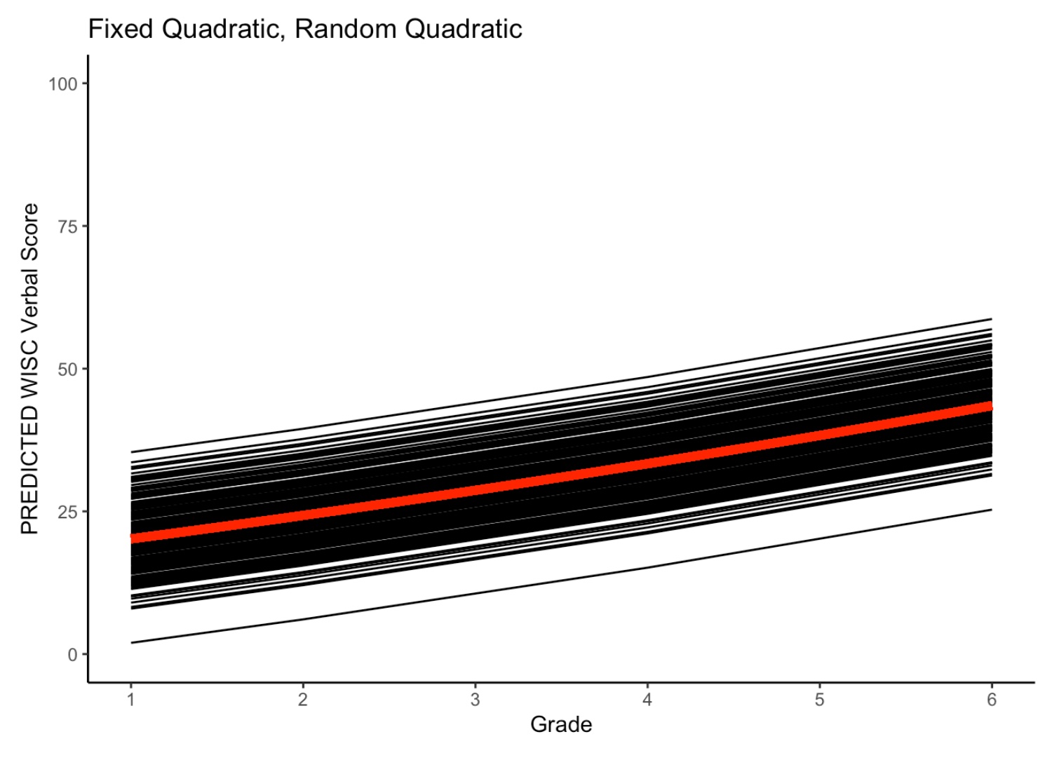
summary(lin_lme)14.1.6 Quadratic Growth Model
Now, let’s review the quadratic growth model. The quadratic growth model accounts for nonlinearity by adding a second-order power of time to the linear growth model.
14.1.7 Quadratic Growth Equations
The quadratic growth model can be written as
\[\begin{align} y_{ti} = & \beta_{0i} + \beta_{1i}\text{time}+ \beta_{2i}\text{time}^{2} + e_{ti}, & e_{ti} \sim \mathcal{N}(0,\sigma^{2}_{e}) && \: [\text{Level 1}] \\ \beta_{0i} = & \gamma_{00} + u_{0i}, & u_{0i} \sim \mathcal{N}(0,\sigma^{2}_{u0}) && \: [\text{Level 2}] \\ \beta_{1i} = & \gamma_{10} + u_{1i}, & u_{1i} \sim \mathcal{N}(0,\sigma^{2}_{u1}) && \: \\ \beta_{2i} = & \gamma_{20} + u_{2i}, & u_{2i} \sim \mathcal{N}(0,\sigma^{2}_{u2}) && \: \\ y_{ti} = & \underbrace{\gamma_{00} + \gamma_{10}\text{time} + \gamma_{20}\text{time}^2}_{fixed} + \underbrace{u_{0i} + u_{1i}\text{time} + u_{2i}\text{time}^{2}}_{random} + e_{ti}, & && \: [\text{Combined}] \end{align}\]
where
\[\begin{align} u_{0i}, u_{1i} \sim \left( \left[\begin{array}{r} 0 \\ 0 \\ 0 \end{array}\right], \left[\begin{array}{c} \sigma^{2}_{u0} & \\ \sigma^{2}_{u1u0} & \sigma^{2}_{u1} \\ \sigma^{2}_{u2u0} & \sigma^{2}_{u2u1} & \sigma^{2}_{u2}\\ \end{array}\right]\right), \end{align}\]
and
- \(y_{ti}\) is the repeated measures score for individual \(i\) at time \(t\)
- \(\beta_{0i}\) is the random intercept for individual \(i\)
- predicted score for individual \(i\) when \(\text{time}=0\)
- \(\beta_{1i}\) is the random linear component for individual \(i\)
- the linear component of change or the rate of change when \(\text{time}=0\)
- \(\beta_{2i}\) is the random quadratic component for individual \(i\)
- the quadratic component of change or acceleration (how quickly the rate of change is changing)
- \(\text{time}\) represents time and could be grade, age, year, etc.
- predicted rate of change for individual \(i\) with a 1-unit change in \(\text{time}\)
- \(c_{1}, c_{2}\) have been dropped (set to \(1\)) to simplify notation
- \(e_{it}\) is the time-specific residual score (within-person deviation)
- \(\gamma_{00}\) is the fixed effect for the intercept component
- \(\gamma_{10}\) is the fixed effect for the linear component
- \(\gamma_{20}\) is the fixed effect for the quadratic component
- \(u_{0i}\) is individual \(i\)’s deviation from the intercept component
- \(u_{1i}\) is individual \(i\)’s deviation from the linear component
- \(u_{2i}\) is individual \(i\)’s deviation from the quadratic component
14.1.7.1 Quadratic Growth Code
Here, we present code for fitting the quadratic growth model in the nlme package using both compact and detailed model syntax.
verblong$gradeSquared <- (verblong$grade)^2

quad_nlme <- nlme::nlme(
  verb ~ (gamma_00 + u_0i) + (gamma_10 + u_1i)*grade + (gamma_20 + u_2i)*gradeSquared,
  data = verblong,
  fixed = gamma_00 + gamma_10 + gamma_20~1,
  random = u_0i + u_1i + u_2i~1,
  group = ~id,
  na.action="na.omit",
  start = c(gamma_00 = 20, gamma_10=10, gamma_20=1)
)
summary(quad_nlme)


quad_lme <- nlme::lme(
  fixed = verb ~ 1 + grade + gradeSquared,
  random = ~ 1 + grade|id + gradeSquared|id,
  data=verblong,
  na.action = na.exclude,
  method = "REML" # does not converge with ML
)
summary(quad_lme)