12.4 Unconditional Means Model

It is often recommended to fit the unconditional means model before moving on to more complicated models.

This is primarily because the unconditional means model does well at partitioning variance of the outcome across levels.

We can use this model to better understand the amount of outcome variation that exists at the within and between levels of our model.

If we fail to find sufficient variation at a given level there may be little reason to proceed with attempts to explain variance at that level of analysis.

12.4.1 Level 1

First, let us write out the level-1 (individual) model

\[ y_{it} = 1\beta_{0i} + e_{it} \] where

\(y_{it}\) is the repeated measures score for individual \(i\) at time \(t\)
\(\beta_{0i}\) is the random intercept for individual \(i\) (person-specific mean)
\(e_{it}\) is the time-specific residual score (within-person deviation)
- \(e_{it} \sim \mathcal{N}(0,\sigma^{2}_{e})\)

Note, the level 1 model shows us the true individual-level trajectories are completely flat, sitting at \(\beta_{0i}\).

12.4.2 Level 2

The level-2 (sample) equation for the random intercept \(\beta_{0i}\) can be written as

\[ \beta_{0i} = 1\gamma_{00} + u_{0i} \]

where

\(\gamma_{00}\) is the sample mean for the intercept (grand mean)
\(u_{0i}\) is individual \(i\)’s deviation from the sample mean (between person deviation)
- \(u_{0i} \sim \mathcal{N}(0,\psi_{u0})\)

Note, the looking at the level 1 and level 2 model tells us that while these flat trajectories may differ in elevation, across everyone in the population, their average elevation is \(\gamma_{00}\).

12.4.3 Single Equation

We can write also both models in a single equation as follows

\[ y_{it} = (1\gamma_{00} + 1u_{0i}) + e_{it} \] where

\(y_{it}\) is the repeated measures score for individual \(i\) at time \(t\)
\(\gamma_{00}\) is the sample mean for the intercept (grand mean)
\(u_{0i}\) is individual \(i\)’s deviation from the sample mean (between person deviation)
- \(u_{0i} \sim \mathcal{N}(0,\psi_{u0})\)
\(e_{it}\) is the time-specific residual score (within-person deviation)
- \(e_{it} \sim \mathcal{N}(0,\sigma^{2}_{e})\)

12.4.4 Model Elaboration

12.4.4.1 Within-Person Residual Covariance

For clarity, Let’s write out the full variance covariance matrix of the within-person residuals (spanning across the \(T = 3\) repeated measures). Remember, we wrote \((e_{it} \sim \mathcal{N}(0,\sigma^{2}_{e}))\), or in matrix notation,

\[ \sigma^{2}_{e}\boldsymbol{I} = \sigma^{2}_{e} \left[\begin{array} {rrr} 1 & 0 & 0 \\ 0 & 1 & 0 \\ 0 & 0 & 1 \end{array}\right] = \left[\begin{array} {rrr} \sigma^{2}_{e} & 0 & 0 \\ 0 & \sigma^{2}_{e} & 0 \\ 0 & 0 & \sigma^{2}_{e} \end{array}\right] = \boldsymbol{\Lambda} \] Note, this is the homoscedasticity of errors assumption.

12.4.4.2 Between-Person Residual Covariance

We can now do the same for the full variance covariance matrix of the between-person residuals,

\[ \left[\begin{array} {r} \psi_{u0} \end{array}\right] = u_{0i}u_{0i}' \]

Note, in the unconditional means model there is no-growth, each individual has an intercept, but no change in scores is predicted because there are no predictors (e.g. time) in the level-1 equation.

12.4.5 Estimated Quantities

Importantly, in the unconditional means model we will be interested in estimating three parameters:

The sample-level mean of the random intercept (\(\gamma_{00}\)) or the grand mean across all occasions and individuals.
The variance of the random intercept (\(\psi_{u0}\))
- Provides information about the magnitude of between person differences in scores at each measurement occasion.
The residual variance (\(\sigma^{2}_{e}\))
- Provides information about the magnitude of with-person fluctuations in scores over time.

12.4.6 More Notation

It is also worth mentioning that through some replacement (e.g., replacing \(u_{i}\) = \(b_{i}\), the different vectors of 1 with \(X_{i}\) and \(Z_{i}\) = 1 we can get to … \[ \boldsymbol{Y} = \boldsymbol{X}\boldsymbol{\beta} + \boldsymbol{Z}\boldsymbol{b} + \boldsymbol{e} \] which is just the more general notation often used in the statistics literature. The equation we started with, with another multilevel notation … \[ \boldsymbol{Y} = \boldsymbol{X}\boldsymbol{\gamma} + \boldsymbol{Z}\boldsymbol{u} + \boldsymbol{e} \]

12.4.7 Unconditional Means Model in R

We can write the unconditional means model in R as follows.

um_fit <- lme(
  fixed = verb ~ 1, 
  random = ~ 1|id, 
  data = verblong,
  na.action = na.exclude
)
summary(um_fit)

## Linear mixed-effects model fit by REML
##   Data: verblong 
##       AIC      BIC   logLik
##   4682.66 4695.906 -2338.33
## 
## Random effects:
##  Formula: ~1 | id
##         (Intercept) Residual
## StdDev:    4.406063   10.277
## 
## Fixed effects:  verb ~ 1 
##                Value Std.Error  DF  t-value p-value
## (Intercept) 33.92433 0.5174359 408 65.56238       0
## 
## Standardized Within-Group Residuals:
##        Min         Q1        Med         Q3        Max 
## -1.9626206 -0.6924771 -0.1481960  0.5511044  3.1026127 
## 
## Number of Observations: 612
## Number of Groups: 204

# um_fit2 <- lmer(
#   verb ~ 1 + (1|id),
#   data=verblong,
#   na.action = na.exclude
# )
# summary(um_fit2)

12.4.7.1 Interpretation

The single fixed effect in our unconditional means model is the grand mean, or \(\gamma_{00}\). Rejection of the null indicates the average verbal score between Grades 2 and 6 is non-zero.

Next we look at the random effects. The estimated between-person standard deviation is \(\psi_{u0}=4.4\) and the estimated within-person standard deviation is \(\sigma^{2}_{e}=10.28\).

12.4.8 Intra-Class Correlation

The intra-class correlation (ICC) as the ratio of the random intercept variance (between-person) to the total variance, defined as the sum of the random intercept variance and residual variance (between + within). Specifically, \[ICC_{between} = \frac{\sigma^{2}_{u0}}{\sigma^{2}_{u0} + \sigma^{2}_{e}}\]

12.4.8.1 Calculating the ICC

The ICC is the ratio of the random intercept variance (between-person var) over the total variance (between + within var):

ICC_between <- 4.4^2 / (4.4^2 + 10.28^2)
ICC_between

## [1] 0.1548324

# Simple function for computing ICC from lme() output
ICClme <- function(out) {
   varests <- as.numeric(VarCorr(out)[1:2])
   return(paste("ICC =", varests[1]/sum(varests)))
}
ICClme(um_fit)

## [1] "ICC = 0.155269768304537"

From the unconditional means model, the ICC was calculated, which indicated that of the total variance in verbal scores, approximately 16%, is attributable to between-person variation whereas 84% is attributable to within-person variation. This means there is a good portion of within-person variance sill to be modeled.

12.4.9 Model-Impled Moments

What is the implied representation of the basic information? What are the model-implied moments?

Let’s remember our original equation.

\[\left[\begin{array} {r} Y_{i0} \\ Y_{i1} \\ Y_{i2} \end{array}\right] = \left[\begin{array} {r} X_{0} \\ X_{1} \\ X_{2} \end{array}\right] \left[\begin{array} {r} \beta_{0} \end{array}\right] + \left[\begin{array} {r} Z_{0} \\ Z_{1} \\ Z_{2} \end{array}\right] \left[\begin{array} {r} u_{0i} \end{array}\right] + \left[\begin{array} {r} e_{i0} \\ e_{i1} \\ e_{i2} \end{array}\right]\]

In this unconditional means model the \(X\) and \(Z\) design matrices are simply vectors of \(1\)s, leaving us with

\[\left[\begin{array} {r} Y_{i0} \\ Y_{i1} \\ Y_{i2} \end{array}\right] = \left[\begin{array} {r} 1 \\ 1 \\ 1 \end{array}\right] \left[\begin{array} {r} \beta_{0} \end{array}\right] + \left[\begin{array} {r} 1 \\ 1 \\ 1 \end{array}\right] \left[\begin{array} {r} u_{0i} \end{array}\right] + \left[\begin{array} {r} e_{i0} \\ e_{i1} \\ e_{i2} \end{array}\right]\].

12.4.9.1 Mean Vector

To obtain the model-implied mean vector we want \(\mathbb{E}(\mathbf{Y})\). Remember, from our covariance algebra

\[ \mathbb{E}(\mathbf{A}+\mathbf{B}+\mathbf{C}) = \mathbb{E}(\mathbf{A}) +\mathbb{E}(\mathbf{B})+\mathbb{E}(\mathbf{C}) \] which gives us

\[\begin{align} \mathbb{E} \left( \left[\begin{array} {r} Y_{i0} \\ Y_{i1} \\ Y_{i2} \end{array}\right] \right) = & \mathbb{E}\left( \left[\begin{array} {r} 1 \\ 1 \\ 1 \end{array}\right] \left[\begin{array} {r} \beta_{0} \end{array}\right] \right) + \mathbb{E}\left( \left[\begin{array} {r} 1 \\ 1 \\ 1 \end{array}\right] \left[\begin{array} {r} u_{0i} \end{array}\right] \right) + \mathbb{E}\left( \left[\begin{array} {r} e_{i0} \\ e_{i1} \\ e_{i2} \end{array}\right] \right) \end{align}\]

or after simplifying

\[\begin{align} \mathbb{E} \left( \mathbf{Y} \right) = & \mathbb{E}\left( \beta_{0}\right) + \mathbf{0} + \mathbf{0} \\ \end{align}\]

12.4.9.2 Mean Vector in R

Let’s make the implied mean vector in R.

First, extract the fixed effects from the model using fixef(), specifically the contents of the \(\beta\) matrix.

fixef(um_fit)

## (Intercept) 
##    33.92433

beta <- matrix(fixef(um_fit)[1], nrow = 1, ncol = 1)
beta

##          [,1]
## [1,] 33.92433

Create the model design matrix for the fixed effects. In this model this is a matrix of order \(3 \times 1\).

X <- matrix(c(1,1,1), nrow = 3, ncol = 1)
X

##      [,1]
## [1,]    1
## [2,]    1
## [3,]    1

Creating the model implied mean vector through multiplication

\[ \mathbf{Y} = \mathbf{X}\mathbf{\beta} + 0 + 0 \]

meanvector_um <- X %*% beta
meanvector_um

##          [,1]
## [1,] 33.92433
## [2,] 33.92433
## [3,] 33.92433

Note this is the overall (grand) mean.

12.4.9.3 Model-Implied Covariance Matrix

Now, let’s take a look at the model-implied variance-covariance matrix. Before we start let’s review the model again,

\[ \boldsymbol{Y}_i = \boldsymbol{X}_i\boldsymbol{\beta} + \boldsymbol{Z}_i\boldsymbol{u}_i + \boldsymbol{e}_i \]

where

\(\mathbf{Z}_i\) is the random effects regressor (design) matrix;
\(\boldsymbol{\beta}\) contains the fixed effects;
\(\boldsymbol{u}_i\) contains the random effects which are distributed normally with \(0\) mean and covariance matrix \(\mathbf{\Psi}\) and
\(\boldsymbol{e}_i\) are errors which are distributed normally with \(0\) mean and covariance matrix \(\mathbf{\Lambda_{i}}\), and
our “standard assumption” was that \(\mathbf{\Lambda_{i}} = \mathbf{\sigma^2}\mathbf{I}\) (homogeneity of errors).

We’d like to identify the quantity \(\mathbb{C}ov(\mathbf{Y})\).

We subtract the “means” from both sides … \[\left[\begin{array} {r} Y_{i0} \\ Y_{i1} \\ Y_{i2} \end{array}\right] - \left[\begin{array} {r} X_{0} \\ X_{1} \\ X_{2} \end{array}\right] \left[\begin{array} {r} \beta_{0} \end{array}\right] = \left[\begin{array} {r} Z_{0} \\ Z_{1} \\ Z_{2} \end{array}\right] \left[\begin{array} {r} u_{0i} \end{array}\right] + \left[\begin{array} {r} e_{i0} \\ e_{i1} \\ e_{i2} \end{array}\right]\]

So on the left side we now have de-meaned scores and on the right we have a between-portion part and a within-person part. Note that \(\mathbf{Y}^{*}\) is now mean-centered, and as such, \(\mathbb{C}ov(\mathbf{Y}) = \mathbf{Y}^{*}\mathbf{Y}^{*'}\).

This gives us

\[\begin{align} \mathbf{Y}^{*} \mathbf{Y}^{*'} = (\mathbf{Z}\mu_{0i} + \boldsymbol{\epsilon})(\mathbf{Z}\mu_{0i} + \boldsymbol{\epsilon})^{'} \\ = (\mathbf{Z}\mu_{0i} + \boldsymbol{\epsilon})(\mu_{0i}^{'}\mathbf{Z}^{'} + \boldsymbol{\epsilon}^{'}) & \quad \text{[Distribute transpose]}\\ = \mathbf{Z}\mu_{0i}\mu_{0i}^{'}\mathbf{Z}^{'} + \mathbf{Z}\mu_{0i}\boldsymbol{\epsilon}^{'} + \boldsymbol{\epsilon}\mu_{0i}^{'}\mathbf{Z}^{'} + \boldsymbol{\epsilon}\boldsymbol{\epsilon}^{'} & \quad \text{[Expand]}\\ = \mathbf{Z}\mu_{0i}\mu_{0i}^{'}\mathbf{Z}^{'} + \boldsymbol{\epsilon}\boldsymbol{\epsilon}^{'} & \quad \text{[Orthogonality]}\\ = \mathbf{Z}\boldsymbol{\Psi}\mathbf{Z}^{'} + \boldsymbol{\Lambda} & \quad \text{[De. \: Covariances]}\\ \end{align}\]

Or we can alternatively see this in matrix form, without recalculating all the steps.

\[\left[\begin{array} {r} Y^*_{i0} \\ Y^*_{i1} \\ Y^*_{i2} \end{array}\right] = \left[\begin{array} {r} Z_{0} \\ Z_{1} \\ Z_{2} \end{array}\right] \left[\begin{array} {r} u_{0i} \end{array}\right] + \left[\begin{array} {r} e_{i0} \\ e_{i1} \\ e_{i2} \end{array}\right]\]

Let’s calculate var-cov matrix …

\[\left[\begin{array} {r} Y^*_{i0} \\ Y^*_{i1} \\ Y^*_{i2} \end{array}\right] \left[\begin{array} {r} Y^*_{i0} & Y^*_{i1} & Y^*_{i2} \end{array}\right] = \left[\begin{array} {r} Z_{0} \\ Z_{1} \\ Z_{2} \end{array}\right] \left[\begin{array} {r} u_{0i} \end{array}\right] \left[\begin{array} {r} u_{0i} \end{array}\right] \left[\begin{array} {r} Z_{0} & Z_{1} & Z_{2} \end{array}\right] + \left[\begin{array} {r} e_{i0} \\ e_{i1} \\ e_{i2} \end{array}\right] \left[\begin{array} {r} e_{i0} & e_{i1} & e_{i2} \end{array}\right]\]

From above we get

\[\left[\begin{array} {r} \hat\Sigma \end{array}\right] = \left[\begin{array} {r} Z_{0} \\ Z_{1} \\ Z_{2} \end{array}\right] \left[\begin{array} {r} \Psi \end{array}\right] \left[\begin{array} {r} Z_{0} & Z_{1} & Z_{2} \end{array}\right] + \left[\begin{array} {r} \sigma^2_{e} \end{array}\right] \left[\begin{array} {r} 1 & 0 & 0 \\ 0 & 1 & 0 \\ 0 & 0 & 1 \end{array}\right]\]

12.4.9.4 Covariance Matrix in R

#parsing the model variances & covariances
VarCorr(um_fit)

## id = pdLogChol(1) 
##             Variance  StdDev   
## (Intercept)  19.41339  4.406063
## Residual    105.61668 10.276997

So, in order to reconstruct the implied variance-covariances, we need to find \(\mathbf{\Psi}\) and \(\mathbf{\sigma^2}\) to create \(\boldsymbol{\Lambda}\), and do some multiplication.

Parse the between-person variances from the model output.

Psi <- matrix(c(as.numeric(VarCorr(um_fit)[1])),nrow = 1, ncol = 1)  
Psi

##          [,1]
## [1,] 19.41339

Create the model design matrix, \(\mathbf{Z}\), for the random effects. In this model this is a matrix of order \(3 \times 1\)

Z <- matrix(c(1,1,1), nrow=3,ncol=1)
Z

##      [,1]
## [1,]    1
## [2,]    1
## [3,]    1

So, the implied variance-covariance matrix of the between-person random effects for the three occasions is:

Cov1 = Z %*% Psi %*% t(Z)
Cov1

##          [,1]     [,2]     [,3]
## [1,] 19.41339 19.41339 19.41339
## [2,] 19.41339 19.41339 19.41339
## [3,] 19.41339 19.41339 19.41339

Which in correlation units implies

Delta = diag(3)
Delta[1,1] = 1/sqrt(Cov1[1,1])
Delta[2,2] = 1/sqrt(Cov1[2,2])
Delta[3,3] = 1/sqrt(Cov1[3,3])
Delta %*% Cov1 %*% Delta

##      [,1] [,2] [,3]
## [1,]    1    1    1
## [2,]    1    1    1
## [3,]    1    1    1

Now, let’s look at the residual error variance-covariance matrix,

sigma2 <- as.numeric(VarCorr(um_fit)[2])
Lambda <- sigma2 * diag(1, nrow = 3, ncol = 3)

Finally, can put the between- and within- pieces together to calculate the model-implied variance-covariance matrix as follows

varcovmatrix_um <- Z %*% Psi %*% t(Z) + (sigma2 * Lambda)
varcovmatrix_um

##             [,1]        [,2]        [,3]
## [1,] 11174.29648    19.41339    19.41339
## [2,]    19.41339 11174.29648    19.41339
## [3,]    19.41339    19.41339 11174.29648

Note, we have a compound symmetry structure in our model-implied covariance matrix.

Together with the implied mean vector, we have the entire picture provided by all the model components.

12.4.10 Model Residuals

Recall what the observed mean and var-cov were …

meanvector

##    verb2    verb4    verb6 
## 25.41534 32.60775 43.74990

varcovmatrix

##          verb2    verb4     verb6
## verb2 37.28784 33.81957  47.40488
## verb4 33.81957 53.58070  62.25489
## verb6 47.40488 62.25489 113.74332

For fun, let’s look at the misfit to the data (observed matrix - model implied matrix)

meanvector - meanvector_um

##           [,1]
## [1,] -8.508987
## [2,] -1.316585
## [3,]  9.825572

varcovmatrix - varcovmatrix_um

##              verb2        verb4        verb6
## verb2 -11137.00864     14.40618     27.99149
## verb4     14.40618 -11120.71578     42.84150
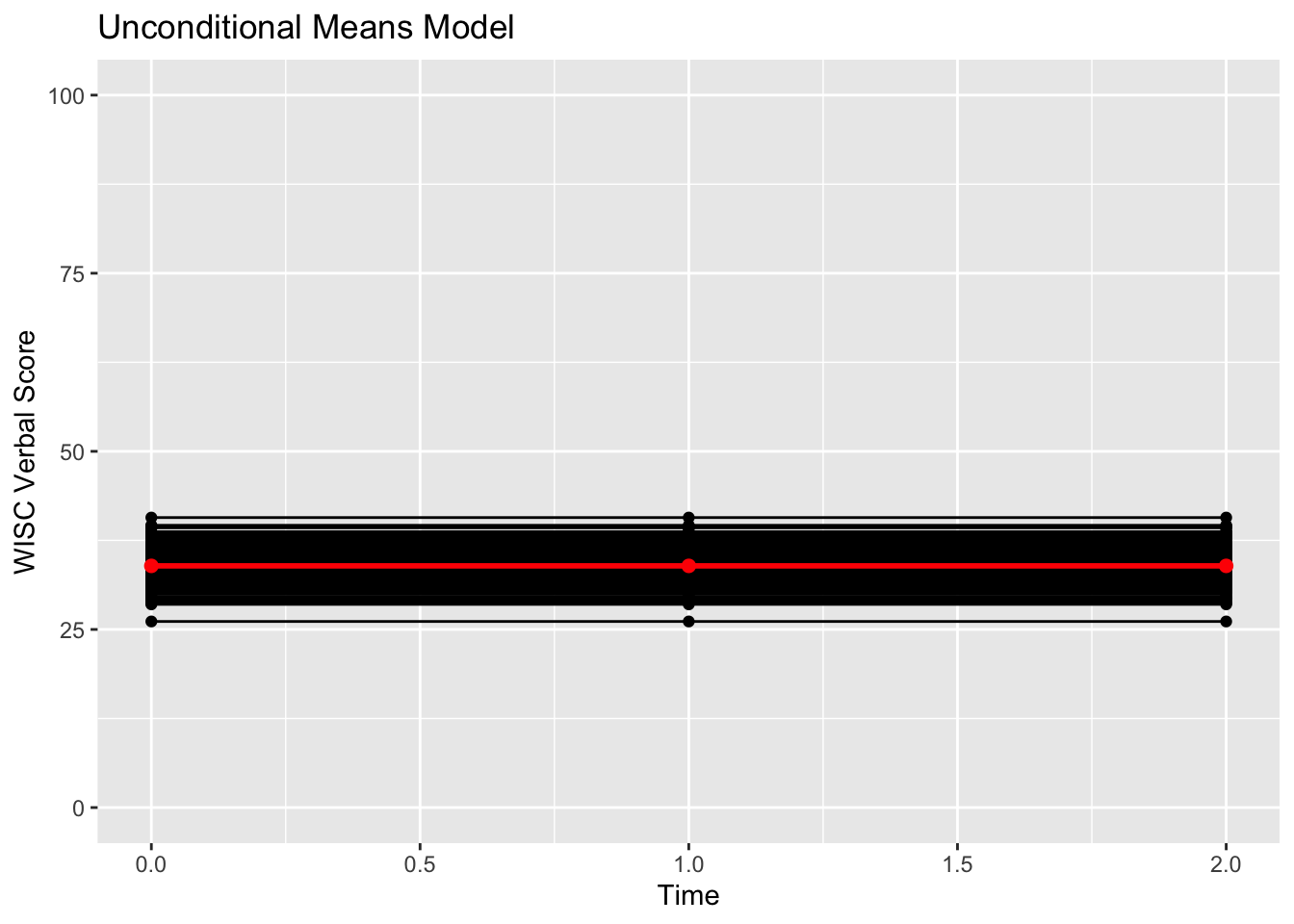
## verb6     27.99149     42.84150 -11060.55317

Fit is not so good. Let’s visualize the implied model.

#Calculating predicted scores from the models 
verblong$pred_um <- predict(um_fit)
#Making the prototype from the implied means
proto_um <- data.frame(cbind(c(1000,1000,1000),c(0,1,2),meanvector_um))
names(proto_um) <- c("id","time0","pred_um")

#plotting implied individual scores
ggplot(data = verblong, aes(x = time0, y = pred_um, group = id)) +
  ggtitle("Unconditional Means Model") +
  geom_point() + 
  geom_line() +
  geom_point(data=proto_um, color="red", size=2) +
  geom_line(data=proto_um, color="red", size=1) +
  xlab("Time") + 
  ylab("WISC Verbal Score") + 
  ylim(0,100) + xlim(0,2)