14.8 Multiphase Growth (Cortisol)

Now let’s consider a multiphase growth model. Multiphase models are based on spline regression models in which two or more regression lines are connected, allowing for the modeling of multiple processes that together may influence intraindividual change over time. For example, consider our data as being potentially characterized by a baseline phase, an intervention phase and a recovery phase.

The multiphase model allows us to articulate how and when each of these intraindividual change processes engages and contributes to the observed scores.

The change points, when one process is “turned off” and another “turned on” are $t = 2$ and $t = 5$. Thus, baseline level process, articulated by the intercept, drive observed levels of cortisol when $t < 2$; the production process, $\text{time}_{1}$, is engaged when $2 ≤ t < 5$, and the dissipation process, $\text{time}_{1}$, is engaged when $t ≥ 5$.

To allow for nonlinearity in the production and dissipation processes we adapt the latent basis GCM presented above to estimate the relevant basis coefficients within each of the multiple intraindividual change process vectors used here.

14.8.1 Equation

The equation for the multiphase model can be written as

\[\begin{align} y_{ti} = & \beta_{0i} + \beta_{1i}\text{time}_{1} + \beta_{2i}\text{time}_{2}+ e_{ti}, & e_{ti} \sim \mathcal{N}(0,\sigma^{2}_{e}) && \: [\text{Level 1}] \\ \beta_{0i} = & \gamma_{00} + u_{0i}, & u_{0i} \sim \mathcal{N}(0,\sigma^{2}_{u0}) && \: [\text{Level 2}] \\ \beta_{1i} = & \gamma_{10} + u_{1i}, & u_{1i} \sim \mathcal{N}(0,\sigma^{2}_{u1}) && \: \\ \beta_{2i} = & \gamma_{20} + u_{2i}, & u_{2i} \sim \mathcal{N}(0,\sigma^{2}_{u2}) && \: \\ y_{ti} = & \gamma_{00} + \gamma_{10}\text{time}_{1} + \gamma_{20}\text{time}_{2}+ u_{0i} + u_{1i}\text{time}_{2} + u_{2i}\text{time}_{2} + e_{ti}, & && \: [\text{Combined}] \end{align}\]

where

\[\begin{align} \text{time}_{1} = & \{0, 0, $alpha_2$, $alpha_3$, 1, 1, 1, 1, 1\}\\ \text{time}_{2} = & \{0, 0, 0, 0, 0, $\alpha_{5}$, $\alpha_{6}$, $\alpha_{7}$, 1}\\ \end{align}\]

and

$y_{ti}$ is the repeated measures score for individual $i$ at time $t$
$\beta_{0i}$ is the random intercept for individual $i$ at $t=0$
- the cortisol level for individual $i$ during baseline
$\beta_{1i}$ is the random slope for individual $i$ during production
$\beta_{2i}$ is the random slope for individual $i$ during recovery
$\text{time}_{1}$ represents the shape factor for the production phase
$\text{time}_{2}$ represents the shape factor for the recovery phase
$e_{it}$ is the time-specific residual score
$\gamma_{00}$ is the fixed-effect for the baseline phase
$\gamma_{10}$ is the fixed-effect for the production phase
$\gamma_{10}$ is the fixed-effect for the recovery phase
$u_{0i}$ is individual $i$’s deviation from the baseline fixed effect
$u_{1i}$ is individual $i$’s deviation from the production fixed effect
$u_{1i}$ is individual $i$’s deviation from the recovery fixed effect

14.8.2 Fit Model

cort_multi <- nlme(cort ~ gamma_00 +
  (0*gamma_10 + 0*gamma_20)*time0 +
  (0*gamma_10 + 0*gamma_20)*time1 +
  (a2*gamma_10 + 0*gamma_20)*time2 +
  (a3*gamma_10 + 0*gamma_20)*time3 +
  (1*gamma_10 + 0*gamma_20)*time4 +
  (1*gamma_10 + a5*gamma_20)*time5 +
  (1*gamma_10 + a6*gamma_20)*time6 +
  (1*gamma_10 + a7*gamma_20)*time7 +
  (1*gamma_10 + 1*gamma_20)*time8,
   fixed = gamma_00 + gamma_10 + gamma_20 + a2 + a3 + a5 + a6 + a7 ~ 1,
   random = gamma_00 + gamma_10 + gamma_20 ~ 1,
   groups =~ id,
   start = c(gamma_00=15,gamma_10=10,gamma_20=-4,
             a2=.4, a3=.5, 
             a5=.7, a6=.8, a7=.9),
   data = cortisol_long,
   na.action = na.exclude,
  control = lmeControl(maxIter = 1e8, msMaxIter = 1e8)
) 
summary(cort_multi)

## Nonlinear mixed-effects model fit by maximum likelihood
##   Model: cort ~ gamma_00 + (0 * gamma_10 + 0 * gamma_20) * time0 + (0 *      gamma_10 + 0 * gamma_20) * time1 + (a2 * gamma_10 + 0 * gamma_20) *      time2 + (a3 * gamma_10 + 0 * gamma_20) * time3 + (1 * gamma_10 +      0 * gamma_20) * time4 + (1 * gamma_10 + a5 * gamma_20) *      time5 + (1 * gamma_10 + a6 * gamma_20) * time6 + (1 * gamma_10 +      a7 * gamma_20) * time7 + (1 * gamma_10 + 1 * gamma_20) *      time8 
##   Data: cortisol_long 
##        AIC      BIC    logLik
##   1412.881 1468.735 -691.4407
## 
## Random effects:
##  Formula: list(gamma_00 ~ 1, gamma_10 ~ 1, gamma_20 ~ 1)
##  Level: id
##  Structure: General positive-definite, Log-Cholesky parametrization
##          StdDev   Corr         
## gamma_00 2.161867 gmm_00 gmm_10
## gamma_10 3.580496 -0.315       
## gamma_20 4.241375 -0.041 -0.286
## Residual 1.535205              
## 
## Fixed effects:  gamma_00 + gamma_10 + gamma_20 + a2 + a3 + a5 + a6 + a7 ~ 1 
##              Value Std.Error  DF  t-value p-value
## gamma_00  5.118082 0.4201167 265 12.18252       0
## gamma_10 14.248891 0.6998856 265 20.35889       0
## gamma_20 -3.797260 0.8089645 265 -4.69398       0
## a2        0.410745 0.0210662 265 19.49782       0
## a3        0.860230 0.0238885 265 36.01023       0
## a5        0.715784 0.0598000 265 11.96963       0
## a6        1.046663 0.0683974 265 15.30267       0
## a7        1.042029 0.0682431 265 15.26937       0
##  Correlation: 
##          gmm_00 gmm_10 gmm_20 a2     a3     a5     a6    
## gamma_10 -0.372                                          
## gamma_20 -0.033 -0.352                                   
## a2       -0.158 -0.032  0.111                            
## a3       -0.033 -0.214  0.205  0.250                     
## a5        0.000  0.059  0.073 -0.056 -0.104              
## a6        0.000 -0.008  0.165  0.007  0.014  0.393       
## a7        0.000 -0.007  0.164  0.006  0.012  0.392  0.504
## 
## Standardized Within-Group Residuals:
##        Min         Q1        Med         Q3        Max 
## -3.4084324 -0.5077968 -0.0178037  0.4909589  3.7024985 
## 
## Number of Observations: 306
## Number of Groups: 34

VarCorr(cort_multi)

## id = pdLogChol(list(gamma_00 ~ 1,gamma_10 ~ 1,gamma_20 ~ 1)) 
##          Variance  StdDev   Corr         
## gamma_00  4.673669 2.161867 gmm_00 gmm_10
## gamma_10 12.819948 3.580496 -0.315       
## gamma_20 17.989264 4.241375 -0.041 -0.286
## Residual  2.356854 1.535205

14.8.3 Predicted Trajectories

#obtaining predicted scores for individuals
cortisol_long$pred_multi <- predict(cort_multi)

#obtaining predicted scores for prototype
cortisol_long$proto_multi <- predict(cort_multi, level=0)


#plotting predicted trajectories
#intraindividual change trajetories
ggplot(data = cortisol_long, aes(x = time, y = pred_multi, group = id)) +
  #geom_point(color="black") + 
  geom_line(color="black") +
  geom_line(aes(x = time, y = proto_multi), color="red",size=2) + 
  xlab("Time") + 
  ylab("Cortisol") + ylim(0,30) +
  scale_x_continuous(breaks=seq(0,8,by=1)) +
  theme_classic()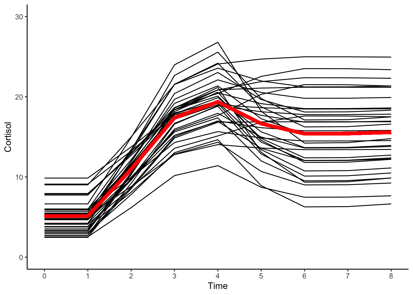

14.8.4 Interpretation

The average baseline cortisol level ($+5.1$); the average amount of cortisol production ($+14.3$); and the average amount by which cortisol declines in the dissipation phase ($–3.8$) can all be read from the fixed effects table.

Looking at the predicted trajectories it is clear the multiphase growth curve model represents the complexity of intraindividual change and interindividual differences in intraindividual change we observed in the raw data.

Furthermore, the model parameters can be understood in a straightforward manner – one in which intraindividual changes in cortisol are characterized by multiple processes, each of which is engaged at know predetermined time in this experimental context.