8.6 Single Predictor Model

OK, let’s include a predictor in our logistic regression model. Let’s start with PersonalSpending such that

\[ logit(\pi_i) = b_0 + b_1PersonalSpending^{*}_{1i} + \epsilon_i \] where \(\pi_i = P(Happy_i = 1)\). Here, \(PersonalSpending^{*}\) is the mean-centered amount of money one spends on themselves in a month (in units of \(100\) dollars).

Let’s fit the model in R.

model10 <- glm(Happy ~ 1 + PersonalSpending_star, 
              family = "binomial", 
              data = dunn2008, 
              na.action = na.exclude)
summary(model10)

## 
## Call:
## glm(formula = Happy ~ 1 + PersonalSpending_star, family = "binomial", 
##     data = dunn2008, na.action = na.exclude)
## 
## Coefficients:
##                        Estimate Std. Error z value Pr(>|z|)    
## (Intercept)           -0.690890   0.084358  -8.190 2.61e-16 ***
## PersonalSpending_star -0.001355   0.004605  -0.294    0.769    
## ---
## Signif. codes:  0 '***' 0.001 '**' 0.01 '*' 0.05 '.' 0.1 ' ' 1
## 
## (Dispersion parameter for binomial family taken to be 1)
## 
##     Null deviance: 805.02  on 631  degrees of freedom
## Residual deviance: 804.93  on 630  degrees of freedom
## AIC: 808.93
## 
## Number of Fisher Scoring iterations: 4

8.6.1 Overdispersion

A quick digression. In the binary logistic regression model overdispersion occurs when the observed variance is larger than what the binomial distribution would predict. For example, if \(Y \sim \mathrm{Binomial}(n_{i},\pi_{i})\), the mean is \(\u_{i}=n_{i}\pi_{i}\) and the variance is \(n_{i}\pi_{i}(1-\pi_{i})\). Since both of these moments rely on \(\pi_{i}\), it can be overly restrictive, and if overdispersion is present inferences can become distorted. We will talk about this more later.

8.6.2 Coefficients

Again, There are essentially three ways to interpret coefficients from a logistic regression model:

The log-odds (or logit)
The Odds
Probabilities

8.6.2.1 Log-Odds

The parameter estimate \(b_0\) reflects the expected log-odds (\(-0.69\)) of being happy for an individual with an average amount of personal spending.

The estimate for \(b_1\) indicates the expected difference of the log-odds of being happy for a \(100\) dollar difference in personal spending. Therefore, we expect a \(-0.001\) difference in the log-odds of being happy for a \(100\) dollar difference in personal spending.

8.6.2.2 Odds

Parameter estimates from a logistic regression are often reported in terms of odds rather than log-odds. To obtain parameters in odds units, we simply exponentiate the coefficients. Note that this is just one of the steps of the inverse link function (which would take us all the way to probability units).

exp(cbind(OR = coef(model10), confint(model10)))

## Waiting for profiling to be done...

##                              OR     2.5 %    97.5 %
## (Intercept)           0.5011299 0.4240750 0.5903901
## PersonalSpending_star 0.9986459 0.9886908 1.0072747

In other words, the odds of being happy when personal spending is at average levels is \(exp(-0.690890) = 0.5\).

In regard to the slope coefficient, for a \(100\) dollar difference in monthly personal spending, we expect to see about \(.1\%\) decrease in the odds of being happy. This decrease does not depend on the value that personal spending is held at. Note this is not significant and we would not report this interpretation in practice. Essentially, if the odds ratio is equal to one, the predictor did not have an impact on the outcome.

8.6.2.3 Probability

Remember, probabilities range from \([0,1]\), whereas log-odds (the output from the raw logistic regression equation) can range from \((-\infty,\infty)\), and odds and odds ratios can range from \((0,\infty)\). Due to the bounded range of probabilities, probabilities are non-linear, but log-odds can be linear.

For example, as personal spending goes up by constant increments, the probability of happiness will increase (decrease) by varying amounts, but the log-odds will increase (decrease) by a constant amount, and the odds will increase (decrease) by a constant multiplicative factor.

For this reason it is not so simple to interpret probabilities in logistic regression from the coefficient directly. Often it is much simpler to plot the probabilities across a range of the predictor variables.

ggplot(data=dunn2008,
       aes(x=PersonalSpending_star,y=Happy)) +
 geom_point(alpha = .08, size = 10) +
 xlab("Personal Spending") +
 ylab("Happy") +
 theme_bw() +
 stat_smooth(method = 'glm', method.args = list(family = "binomial"), se = TRUE)

## `geom_smooth()` using formula = 'y ~ x'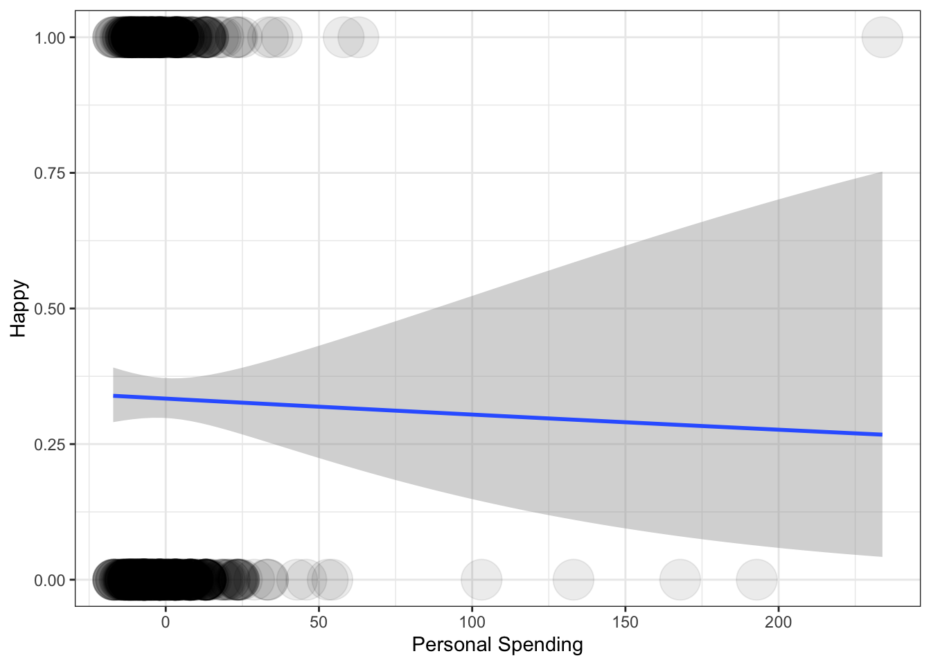

Notice how the density of the observations is visualized by manipulating the transparency (alpha) level of the data points. The predicted curve based on our model has of course a non-linear shape (however, if we were to plot the relationship between the variables with using the logit link, it would be a straight line).