10.4 marginaleffects: Slopes

Slopes are defined as the partial derivatives of the regression equation with respect to an explanatory variable of interest (i.e. a marginal effect or trend). In the remainder of this section we use the terms slope and marginal effect interchangeably.

The marginal effect is a unit- (or person-level) measure of association between changes in a regressor and changes in the response. In a simple linear model the marginal effects will be the same from individual to individual. In anything more complex the marginal effect will vary by individual, because it depends on the values of the other covariates for each individual.

The slopes() function produces unique estimates of the marginal effect for each row of the data used to fit the model. The output of slopes() is a simple data.frame.

library(marginaleffects)
head(slopes(model4))

## 
##         Term Contrast Estimate Std. Error    z Pr(>|z|)   S   2.5 % 97.5 %
##  abuse_freq1    1 - 0    0.590      0.382 1.55    0.122 3.0 -0.1576  1.338
##  abuse_freq1    1 - 0    0.406      0.264 1.54    0.124 3.0 -0.1113  0.923
##  abuse_freq1    1 - 0    0.746      0.482 1.55    0.122 3.0 -0.1984  1.690
##  abuse_freq1    1 - 0    0.625      0.402 1.56    0.119 3.1 -0.1617  1.413
##  abuse_freq1    1 - 0    0.410      0.267 1.54    0.124 3.0 -0.1122  0.933
##  abuse_freq1    1 - 0    0.420      0.263 1.60    0.110 3.2 -0.0955  0.936
## 
## Columns: rowid, term, contrast, estimate, std.error, statistic, p.value, s.value, conf.low, conf.high, predicted_lo, predicted_hi, predicted, morbidityw1, female, health, age, smoke_dose, heavydr2, obese, fampos, friendpos, abuse_rare, abuse_freq1, abuse_freq2 
## Type:  response

Average marginal effects (AME)

To obtain the AMEs we generate predictions for each row of the original data, then collapse to averages.

avg_slopes(model4)

## 
##         Term Contrast Estimate Std. Error      z Pr(>|z|)    S   2.5 %  97.5 %
##  abuse_freq1    1 - 0   0.2521    0.16023  1.573  0.11566  3.1 -0.0620  0.5661
##  abuse_freq2    1 - 0   0.7936    0.16233  4.889  < 0.001 19.9  0.4755  1.1118
##  abuse_rare     1 - 0  -0.0319    0.13557 -0.235  0.81383  0.3 -0.2976  0.2338
##  age            dY/dX   0.0415    0.00424  9.799  < 0.001 72.9  0.0332  0.0498
##  fampos         dY/dX  -0.2399    0.08544 -2.808  0.00498  7.6 -0.4074 -0.0725
##  female         1 - 0   0.8839    0.10324  8.562  < 0.001 56.3  0.6816  1.0863
##  friendpos      dY/dX  -0.1927    0.07665 -2.514  0.01193  6.4 -0.3429 -0.0425
##  health         dY/dX   0.4512    0.11400  3.958  < 0.001 13.7  0.2278  0.6747
##  heavydr2       1 - 0   0.3169    0.12657  2.503  0.01230  6.3  0.0688  0.5649
##  obese          1 - 0   0.7599    0.12066  6.298  < 0.001 31.6  0.5234  0.9964
##  smoke_dose     dY/dX   0.0151    0.00243  6.202  < 0.001 30.7  0.0103  0.0198
## 
## Columns: term, contrast, estimate, std.error, statistic, p.value, s.value, conf.low, conf.high 
## Type:  response

Note that since marginal effects are derivatives, they are only properly defined for continuous numeric variables. When the model also includes categorical regressors, the summary function will try to display relevant (regression-adjusted) contrasts between different categories, as shown above.

Group-Average Marginal Effect (G-AME)

We can also use the by argument the average marginal effects within different subgroups of the observed data, based on values of the regressors.

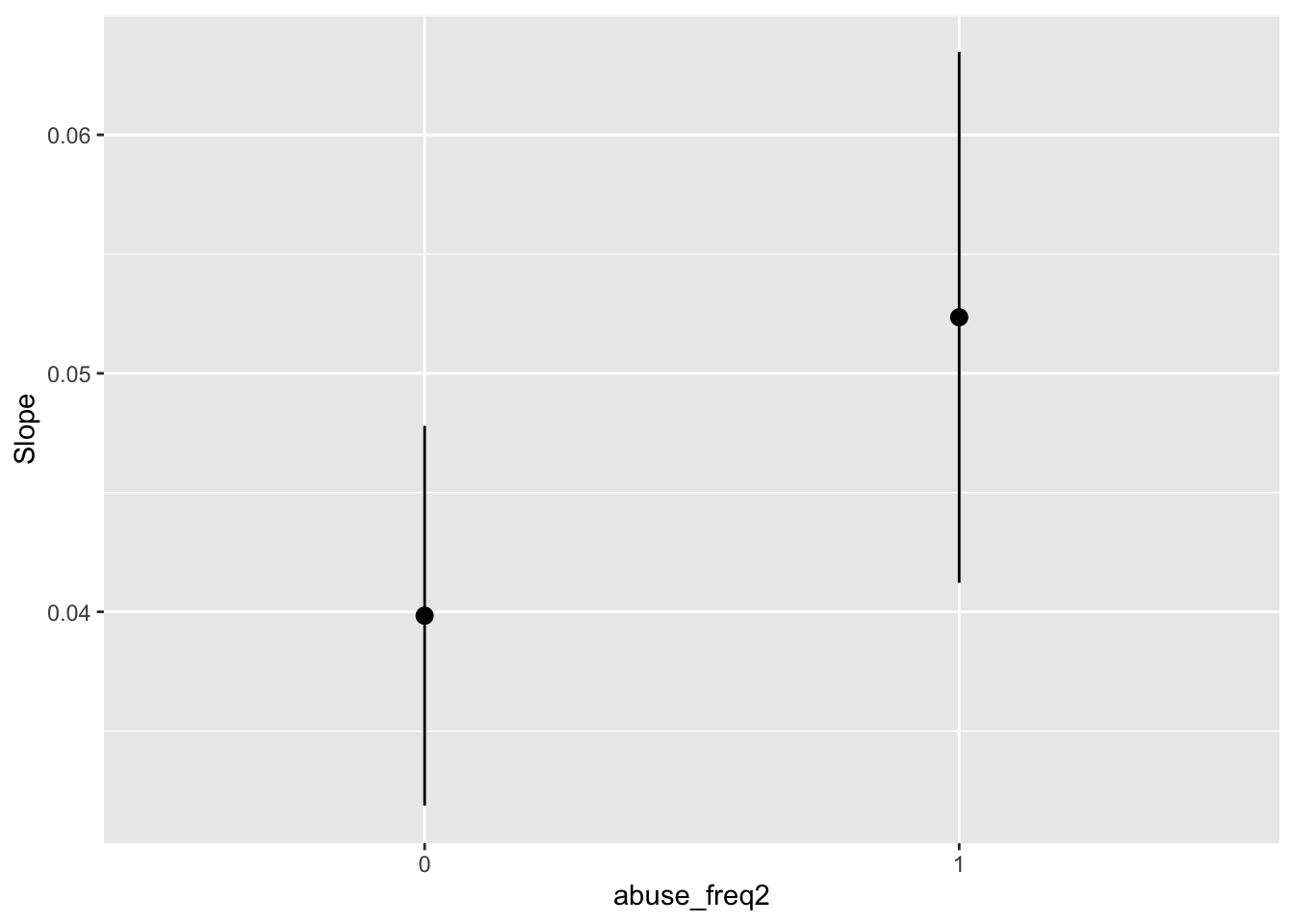
For example, to compute the average marginal effects of age on the number of health problems for those who experienced no childhood maltreatment and those who experienced both physical and emotional abuse:

avg_slopes(
  model4,
  by = "abuse_freq2",
  variables = "age"
)

## 
##  Term    Contrast abuse_freq2 Estimate Std. Error    z Pr(>|z|)    S  2.5 %
##   age mean(dY/dX)           0   0.0384    0.00394 9.74   <0.001 72.1 0.0307
##   age mean(dY/dX)           1   0.0524    0.00556 9.43   <0.001 67.7 0.0415
##  97.5 %
##  0.0461
##  0.0633
## 
## Columns: term, contrast, abuse_freq2, estimate, std.error, statistic, p.value, s.value, conf.low, conf.high, predicted_lo, predicted_hi, predicted 
## Type:  response

We can also plot these slopes:

plot_slopes(
  model4,
  condition = "abuse_freq2",
  variables = "age"
)

Marginal Effect at User-Specified Values

Sometimes, we are only interested in looking at the estimated marginal effects for certain types of individuals, or for user-specified values of the regressors. The datagrid function from marginaleffects allows us to build a data grid containing values that are of interest to us.

For example, let’s look at the effect of experiencing both childhood emotional and physical abuse on the number of adult health problems for a 30-year old male who is obese.

avg_slopes(
  model4,
  variables = "abuse_freq2",
  newdata = datagrid(
    age = 30,
    obese = 1,
    female = 0
  )
)

## 
##         Term Contrast Estimate Std. Error    z Pr(>|z|)    S 2.5 % 97.5 %
##  abuse_freq2    1 - 0     0.59      0.114 5.16   <0.001 21.9 0.366  0.814
## 
## Columns: rowid, term, contrast, estimate, std.error, statistic, p.value, s.value, conf.low, conf.high, predicted_lo, predicted_hi, predicted 
## Type:  response

Hypothesis Tests

We also might be interested in hypothesis tests based on our model. For example, compared to those who did not experience childhood trauma is the effect of experiencing emotional and physical abuse during childhood on adult health problems different depending on whether an individual experienced both, or just one of these type of abuse.

hypotheses(model4, 
  hypothesis = "abuse_freq11 = abuse_freq21"
)

## 
##                         Term Estimate Std. Error     z Pr(>|z|)    S  2.5 %
##  abuse_freq11 = abuse_freq21   -0.183     0.0544 -3.36   <0.001 10.3 -0.289
##  97.5 %
##  -0.076
## 
## Columns: term, estimate, std.error, statistic, p.value, s.value, conf.low, conf.high