11.2 Example Data I
For our first set of examples we will use the WISC data. Here we again read in, subset, and provide basic descriptives.
filepath <- "https://quantdev.ssri.psu.edu/sites/qdev/files/wisc3raw.csv"
wisc3raw <- read.csv(file=url(filepath),header=TRUE)
var_names_sub <- c(
"id", "verb1", "verb2", "verb4", "verb6",
"perfo1", "perfo2", "perfo4", "perfo6",
"momed", "grad"
)
wiscsub <- wisc3raw[,var_names_sub]
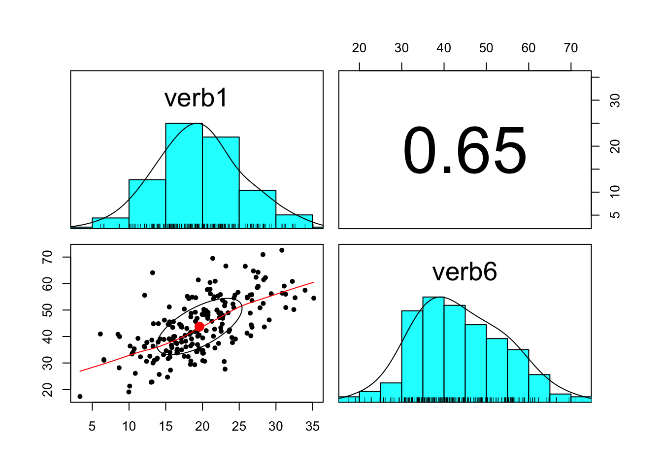
psych::describe(wiscsub)## vars n mean sd median trimmed mad min max range skew
## id 1 204 102.50 59.03 102.50 102.50 75.61 1.00 204.00 203.00 0.00
## verb1 2 204 19.59 5.81 19.34 19.50 5.41 3.33 35.15 31.82 0.13
## verb2 3 204 25.42 6.11 25.98 25.40 6.57 5.95 39.85 33.90 -0.06
## verb4 4 204 32.61 7.32 32.82 32.42 7.18 12.60 52.84 40.24 0.23
## verb6 5 204 43.75 10.67 42.55 43.46 11.30 17.35 72.59 55.24 0.24
## perfo1 6 204 17.98 8.35 17.66 17.69 8.30 0.00 46.58 46.58 0.35
## perfo2 7 204 27.69 9.99 26.57 27.34 10.51 7.83 59.58 51.75 0.39
## perfo4 8 204 39.36 10.27 39.09 39.28 10.04 7.81 75.61 67.80 0.15
## perfo6 9 204 50.93 12.48 51.76 51.07 13.27 10.26 89.01 78.75 -0.06
## momed 10 204 10.81 2.70 11.50 11.00 2.97 5.50 18.00 12.50 -0.36
## grad 11 204 0.23 0.42 0.00 0.16 0.00 0.00 1.00 1.00 1.30
## kurtosis se
## id -1.22 4.13
## verb1 -0.05 0.41
## verb2 -0.34 0.43
## verb4 -0.08 0.51
## verb6 -0.36 0.75
## perfo1 -0.11 0.58
## perfo2 -0.21 0.70
## perfo4 0.59 0.72
## perfo6 0.18 0.87
## momed 0.01 0.19
## grad -0.30 0.03And some bivariate plots of the two-occasion relations.