12.5 Repeated Measures ANOVA
OK, now let’s move to an repeated measures (RM) ANOVA by adding in effects for categorical time. Recall, we must tell R that time0 is a categorical variable using factor()
## Factor w/ 3 levels "0","1","2": 1 2 3 1 2 3 1 2 3 1 ...Here is our RM ANOVA model with time as within-person factor
timecat_fit <- lme(
  fixed = verb ~ 1 + time0,
  random = ~ 1|id,
  data = verblong,
  na.action = na.exclude)
summary(timecat_fit)
## Linear mixed-effects model fit by REML
## Data: verblong
## AIC BIC logLik
## 4013.176 4035.235 -2001.588
##
## Random effects:
## Formula: ~1 | id
## (Intercept) Residual
## StdDev: 6.915667 4.514145
##
## Fixed effects: verb ~ 1 + time0
## Value Std.Error DF t-value p-value
## (Intercept) 25.415343 0.5782155 406 43.95480 0
## time01 7.192402 0.4469670 406 16.09157 0
## time02 18.334559 0.4469670 406 41.01994 0
## Correlation:
## (Intr) time01
## time01 -0.387
## time02 -0.387 0.500
##
## Standardized Within-Group Residuals:
## Min Q1 Med Q3 Max
## -2.61263084 -0.54466998 -0.02451831 0.48627468 3.50536334
##
## Number of Observations: 612
## Number of Groups: 204# timecat_fit2 <- lmer(verb ~ 1 + time0 + (1|id),
# data=verblong,
# na.action = na.exclude)
# summary(timecat_fit2)Remember that interpretation is with respect to time0, with the first category set as default intercept which is
## Factor w/ 3 levels "0","1","2": 1 2 3 1 2 3 1 2 3 1 ...12.5.1 Intra-Class Correlation
The intra-class correlation (ICC) as the ratio of the random intercept variance (between-person) to the total variance, defined as the sum of the random intercept variance and residual variance (between + within). Specifically, \[ICC_{between} = \frac{\sigma^{2}_{u0}}{\sigma^{2}_{u0} + \sigma^{2}_{e}}\]
12.5.1.1 Calculating the ICC
The ICC is the ratio of the random intercept variance (between-person var) over the total variance (between + within var):
# Simple function for computing ICC from lme() output
ICClme <- function(out) {
   varests <- as.numeric(VarCorr(out)[1:2])
   return(paste("ICC =", varests[1]/sum(varests)))
}
ICClme(timecat_fit)
## [1] "ICC = 0.701226878908497"From the current model, the ICC was calculated, which indicated that of the total variance in verbal scores, approximately 70%, is attributable to between-person variation whereas 30% is attributable to within-person variation.
12.5.2 Model-Implied Mean Vector
Let’s be explicit with our model
\[\left[\begin{array} {r} Y_{i0} \\ Y_{i1} \\ Y_{i2} \end{array}\right] = \left[\begin{array} {r} 1 & 0 & 0 \\ 1 & 1 & 0 \\ 1 & 0 & 1 \end{array}\right] \left[\begin{array} {r} \beta_{0} \\ \beta_{1} \\ \beta_{2} \end{array}\right] + \left[\begin{array} {r} 1 \\ 1 \\ 1 \end{array}\right] \left[\begin{array} {r} u_{0i} \end{array}\right] + \left[\begin{array} {r} e_{i0} \\ e_{i1} \\ e_{i2} \end{array}\right]\].
Making the implied mean vector
## (Intercept)      time01      time02
##   25.415343    7.192402   18.334559
beta <- matrix(
c(
fixef(timecat_fit)[1],
fixef(timecat_fit)[2],
fixef(timecat_fit)[3]
), nrow =3, ncol=1)
beta## [,1]
## [1,] 25.415343
## [2,] 7.192402
## [3,] 18.334559Create the model design matrix for the fixed effects. In this model this is a matrix of order \(3 \times 3\).
##      [,1] [,2] [,3]
## [1,]    1    0    0
## [2,]    1    1    0
## [3,]    1    0    1
Creating the model implied mean vector through multiplication
\[ \mathbf{Y} = \mathbf{X}\mathbf{\beta} + 0 + \]
##          [,1]
## [1,] 25.41534
## [2,] 32.60775
## [3,] 43.74990
See the differences in the means across levels of time0.
12.5.3 Model-Implied Covariance Matrix
Making the implied variance-covariance matrix.
## id = pdLogChol(1)
##             Variance StdDev
## (Intercept) 47.82645 6.915667
## Residual    20.37751 4.514145
From this, we need to create the model implied variance-covariance.
Parse the between-person variances from the model output.
##          [,1]
## [1,] 47.82645
Create the model design matrix for the random effects. In this model this is a matrix of order \(3 \times 1\)
##      [,1]
## [1,]    1
## [2,]    1
## [3,]    1
So, the implied variance-covariance matrix of the between-person random effects for the three occasions is:
##          [,1]     [,2]     [,3]
## [1,] 47.82645 47.82645 47.82645
## [2,] 47.82645 47.82645 47.82645
## [3,] 47.82645 47.82645 47.82645
Next, we parse the residual/“error” variance-covariance.
So the residual within-person residual/“error” structure
##          [,1]     [,2]     [,3]
## [1,] 20.37751  0.00000  0.00000
## [2,]  0.00000 20.37751  0.00000
## [3,]  0.00000  0.00000 20.37751
As before, we have homogeneity and uncorrelated errors.
Finally, calculate the implied variance-covariances of total model
##          [,1]     [,2]     [,3]
## [1,] 68.20396 47.82645 47.82645
## [2,] 47.82645 68.20396 47.82645
## [3,] 47.82645 47.82645 68.20396
Again, notice the compound symmetry structure.
For fun, let’s look at the misfit (real matrix - model implied)
##               [,1]
## [1,]  7.105427e-15
## [2,] -6.394885e-14
## [3,] 4.973799e-14## verb2 verb4 verb6
## verb2 -30.9161173 -14.00688 -0.4215677
## verb4 -14.0068803 -14.62326 14.4284384
## verb6 -0.4215677 14.42844 45.5393553The means are now perfectly reproduced, however, the variances and covariances are not so good, particularly the variances
Let’s make a picture of the implied model.
#Calculating predicted scores from the models
verblong$pred_timecat <- predict(timecat_fit)
#Making the prototype from the implied means
proto_timecat <- data.frame(cbind(c(1000,1000,1000),c(0,1,2),meanvector_timecat))
names(proto_timecat) <- c("id","time0","pred_timecat")

#need to convert time0 back into a continuous variable for plotting as intraindividual change
verblong$time0 <- as.numeric(unclass(verblong$time0))-1
#plotting implied individual scores
ggplot(data = verblong, aes(x = time0, y = pred_timecat, group = id)) +
  ggtitle("RM ANOVA Model (time categorical)") +
  geom_point() +
  geom_line() +
  geom_point(data=proto_timecat, color="red", size=2) +
  geom_line(data=proto_timecat, color="red", size=1, linetype=2) +
  xlab("Time") +
  ylab("WISC Verbal Score") +
  ylim(0,100) + xlim(0,2) +
  theme_classic()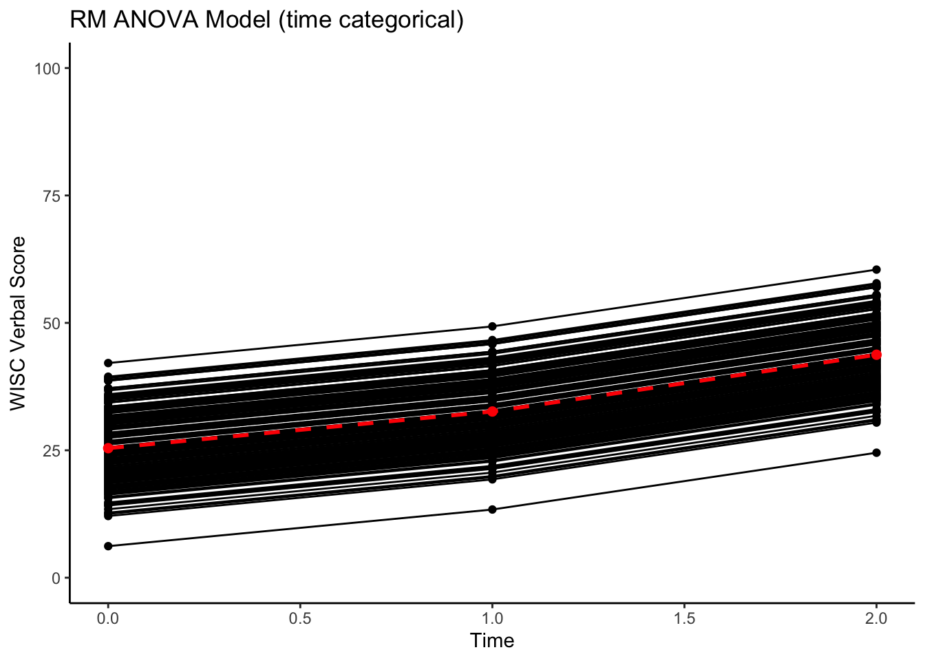
Notice that the implied lines are all parallel. This is a model of mean differences.
Can also see what the residuals look like.
#Calculating residual scores from the models
verblong$resid_timecat <- residuals(timecat_fit)

#plotting implied individual scores
ggplot(data = verblong, aes(x = time0, y = resid_timecat, group = id)) +
  ggtitle("RM ANOVA Model Residuals (time categorical)") +
  geom_point() +
  xlab("Time") +
  ylab("WISC Verbal Score") +
  xlim(0,2) +
  theme_classic()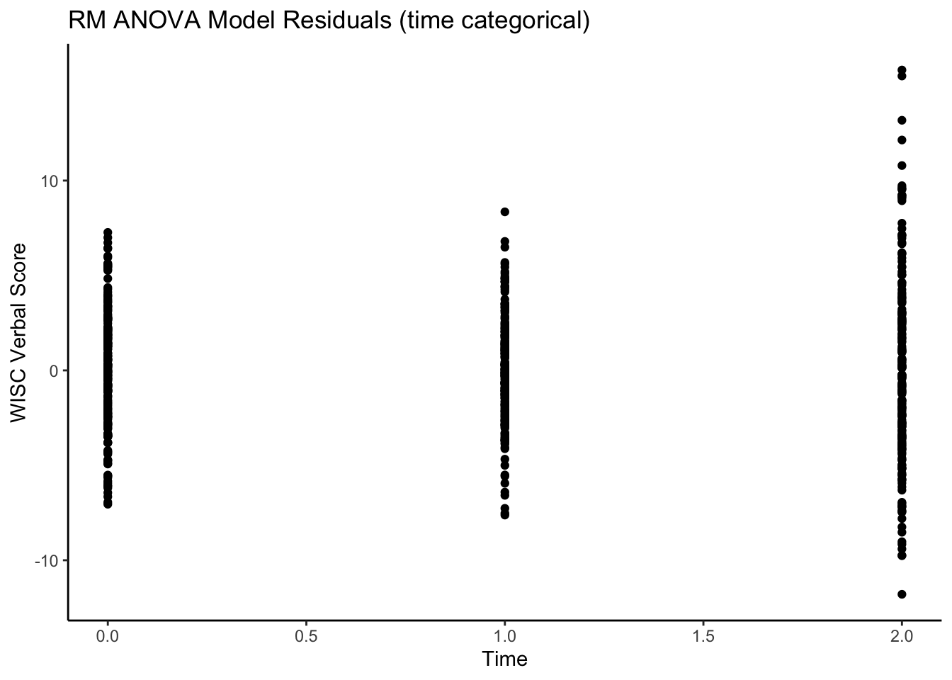
Note, that the points are not connected - this is to highlight the model and the implication that the within-person residuals are from the occasion-specific mean (NOT from a trajectory).Note also the heteroskedasticity of the residuals.