3.3 Describing Covariances
In the previous section we looked at the means and variances. Because these are repeated measures, we can also look at covariances and correlations over time. A simple covariance and correlation matrix of the verbal scores across grades can be produced using the cov() and cor() function.
##          verb1    verb2    verb4     verb6
## verb1 33.72932 25.46388 30.88886  40.51478
## verb2 25.46388 37.28784 33.81957  47.40488
## verb4 30.88886 33.81957 53.58070  62.25489
## verb6 40.51478 47.40488 62.25489 113.74332## verb1 verb2 verb4 verb6
## verb1 1.0000000 0.7180209 0.7265974 0.6541040
## verb2 0.7180209 1.0000000 0.7566242 0.7279080
## verb4 0.7265974 0.7566242 1.0000000 0.7974552
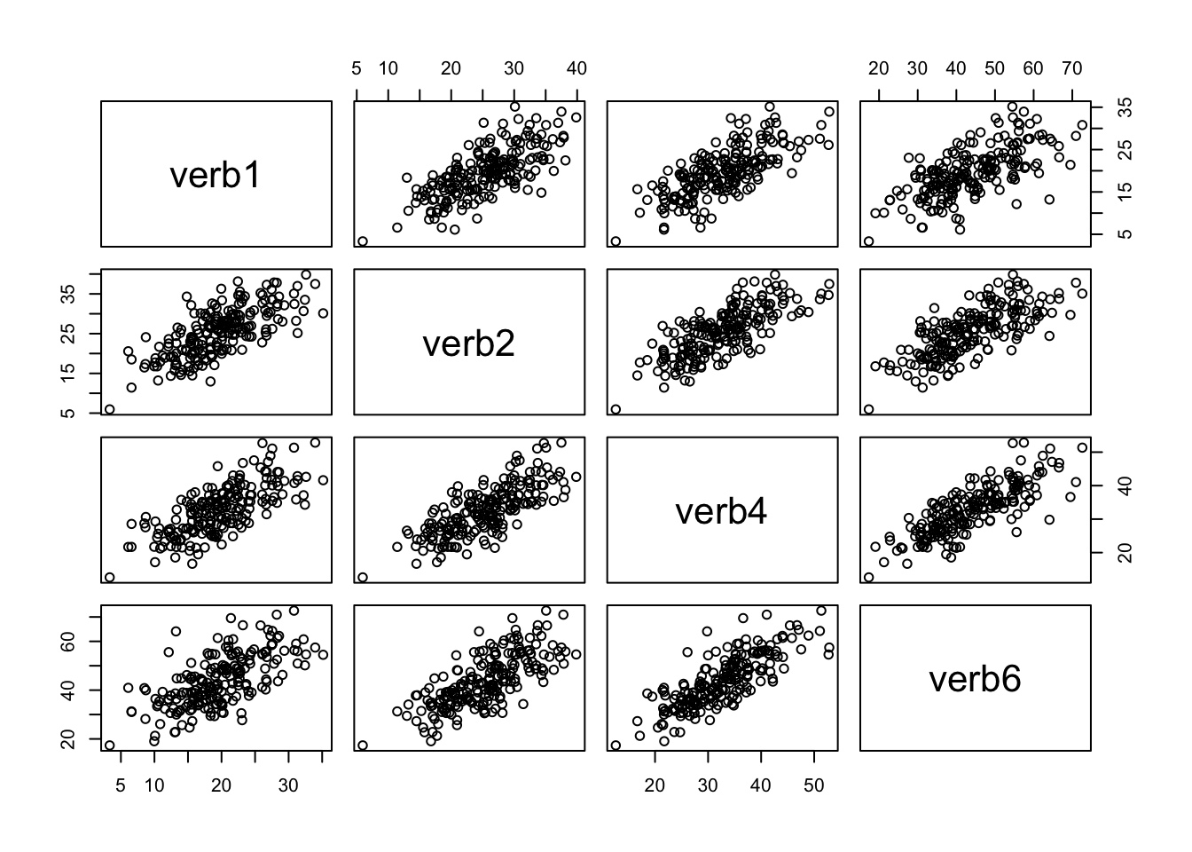
## verb6 0.6541040 0.7279080 0.7974552 1.0000000A plot corresponding to the correlation matrix can be obtained in a number of different ways. First, using the pairs() function from base R.
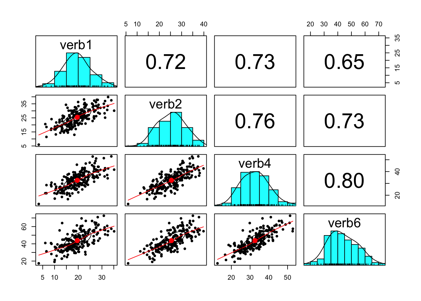
There is also a pairs.panel() function in the psych package. Here we see a LOESS smoothed fit line in red.
Finally, thescatterplotMatrix() from the car (Fox and Weisberg 2019) package can be used to create scatterplot matrices with confidence bands around the line of best fit.
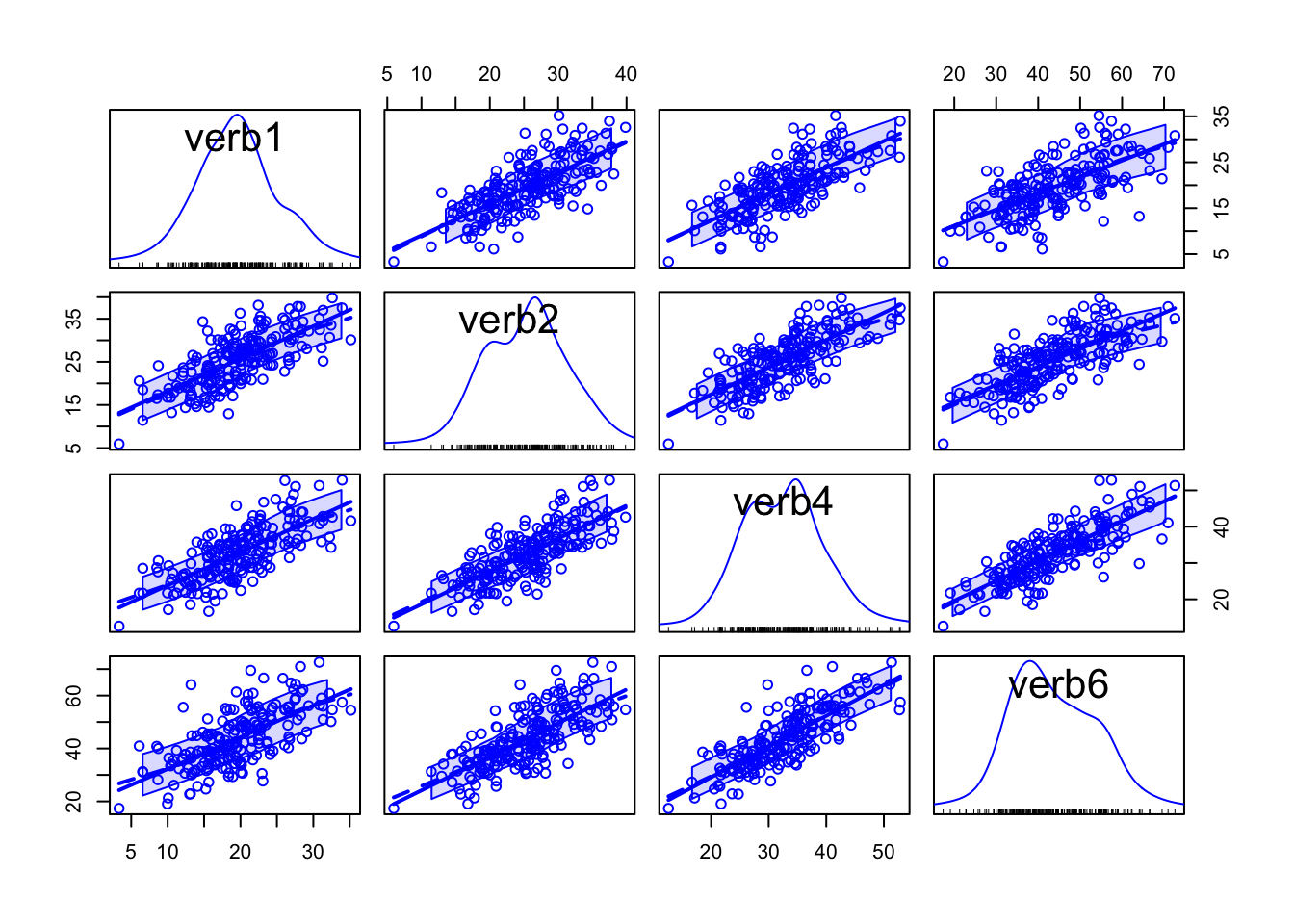
Each of these functions can be customized with additional features. Those interested in specifics should consult the help documentation for each function (e.g. ?car::scatterplotMatrix). It is also worth noting the default behavior of these functions is to provide automatic, data-based ranges for each pair of variables separately.