11.4 Autoregressive Model
Before introducing the model behind each approach is is helpful to consider the data characteristics underlying each notion of change.
Residualized Change
The first approach uses the measure at the second time point as a dependent variable regressed on the the measure at the first time point.
The term residualized change comes from the fact that an outcome, such as verbal scores at grade 6, is regressed on itself at a prior occasion, verbal scores at grade 1. Any variability in the outcome that is explained by the lagged regressor will be set aside and is threfore not explainable by a key predictor.
Thus, the autoregressive effect residualizes the outcome leaving only variability that is unexplained by the lagged variable, which can be construed as the variability due to change.
In this way it is helpful to view the data as a scatter plot, like we would in a regression model.
library("ggplot2")
ggplot(data = wiscsub, aes(x = verb1, y = verb6)) +
  geom_point() +
  xlab("Verbal Scores at Grade 1") +
  ylab("Verbal Scores at Grade 6") +
  theme_bw()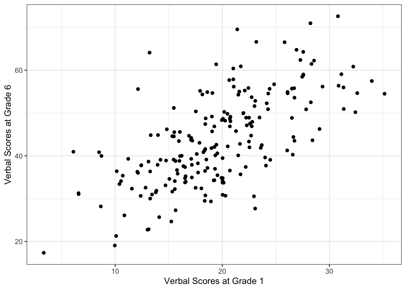
Autoregressive Model
When researchers refer to the autoregressive (residualized change) model for two occasion data they are referring to the following multiple regression model:
\[ y_{2i} = \beta_0 + \beta_1y_{1i} + e_{i} \]
where
- \(y_{1i}\) is the value of the outcome variable for individual \(i\) at time \(1\)
- \(y_{2i}\) is the value of the outcome variable for individual \(i\) at time \(2\)
- \(\beta_0\) is an intercept parameter, the expected value of \(y_{2i}\) when \(y_{1i}=0\)
- \(\beta_1\) is a regression parameter indicating the difference in the predicted score of \(y_{2i}\) based on a 1-unit difference in \(y_{1i}\)
- \(e_{i}\) is the model error for individual \(i\)
Note, the term residualized change comes from the fact that the autoregressive effect residualizes the outcome.
This leaves only the variability that is unexplained by the previous timepoint, or the variability due to change.
Autoregressive Residuals
With the autoregressive model it is helpful to think more about the residual term. Let’s ignore the scaling constant for now,
If we subtract \(\beta_1y_{1i}\) from both sides of the AR equation we isolate the residuals:
\[ e_{i} = y_{2i} -\beta_1y_{1i} \]
Here, the residualized change is the function of a weighted combination of our time 1 scores.
Instead of talking about raw change we are instead asking
“Where would we predict you to be at time 2 given your standing relative to the mean at time 1?”**
Consider the following scenarios:
- \(e_{i}\) is positive: you changed more in a positive direction than would have been expected.
- \(e_{i}\) is negative: you changed more in a negative direction than would have been expected.
Autoregressive Model in R
As we said previously, the autoregrssive model is useful for examining questions about change in interindividual differences. The model for verbal scores at grade 6 can be written as
\[ verb6_{i} = \beta_{0} + \beta_{1}verb1_{i} + e_{i}\]
We note that this is a model of relations among between-person differences. This model is similar to, but is not a single-subject time-series model (which are also called autoregressive models, but are fit to a different kind of data).
Translating the between-person autoregressive model into code and fitting it to the two-occasion WISC data we have
##
## Call:
## lm(formula = verb6 ~ 1 + verb1, data = wiscsub, na.action = na.exclude)
##
## Residuals:
##      Min       1Q   Median       3Q      Max
## -20.2459  -5.8651   0.1781   4.9048  27.9976
##
## Coefficients:
##             Estimate Std. Error t value Pr(>|t|)
## (Intercept) 20.22485    1.99608   10.13   <2e-16 ***
## verb1        1.20117    0.09773   12.29   <2e-16 ***
## ---
## Signif. codes:  0 '***' 0.001 '**' 0.01 '*' 0.05 '.' 0.1 ' ' 1
##
## Residual standard error: 8.087 on 202 degrees of freedom
## Multiple R-squared:  0.4279, Adjusted R-squared:  0.425
## F-statistic: 151.1 on 1 and 202 DF,  p-value: < 2.2e-16
The intercept term, \(\beta_{0}\) = 20.22 is the expected value of Verbal Ability at the 2nd occasion, for an individual with a Verbal Ability score = 0 at the 1st occasion.
The slope term, \(\beta_{1}\) = 1.20 indicates that for every 1-point difference in Verbal Ability at the 1st occasion, we expect a 1.2 point difference at the 2nd occasion.
We can plot the autoregressive model prediction with confidence intervals (CI).
The function termplot takes the fitted lm object. The CI bounds are plotted with the se option and residuals with partial.resid option.
termplot(ARfit,se=TRUE,partial.resid=TRUE,
         main="Autoregressive Model",
         xlab="Verbal Score at Grade 1",
         ylab="Verbal Score at Grade 6")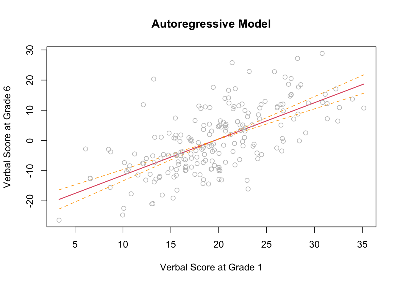
Note that this code makes use of the lm() model object.
We can also do something similar with the raw data using ggplot.
ggplot(data = wiscsub, aes(x = verb1, y = verb6)) +
  geom_point() +
  geom_smooth(method="lm", formula= y ~ 1 + x,
              se=TRUE, fullrange=TRUE, color="red", size=2) +
  xlab("Verbal Score at Grade 1") +
  ylab("Verbal Score at Grade 6") +
  ggtitle("Autoregressive Model") +
  theme_classic()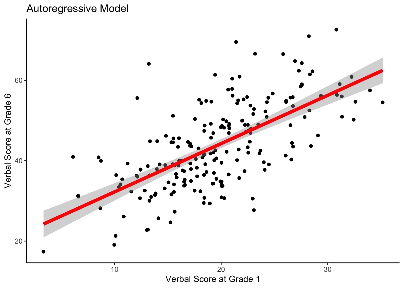
Note that this code embeds an lm() model within the ggplot function.