3.4 Individual-Level Descriptives
Note that our interest is often in individual development, rather than sample development. We need to consider how each individual is changing over time. Thus, we are interested in verbal ability across Time for each individual person. Visualization is typically our best tool for synthesizing the large amounts of information in individual-level data.
ggplot(data = wisclong, aes(x = grade, y = verb, group = id)) +
  geom_point() +
  geom_line() +
  scale_x_continuous(breaks=seq(1,6,by=1)) +
  ylim(0,80) +
  ggtitle("Verbal Ability Score (across grades 1, 2, 4, 6)") +
  xlab("Grade") +
  ylab("Verbal Ability Score") +
  theme_bw() +
  theme(
    panel.grid.major = element_blank(),
    panel.grid.minor = element_blank(),
    strip.background = element_blank()
  )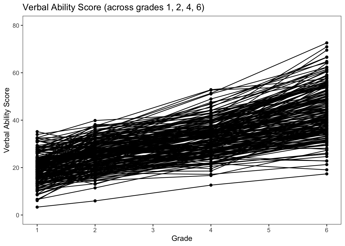
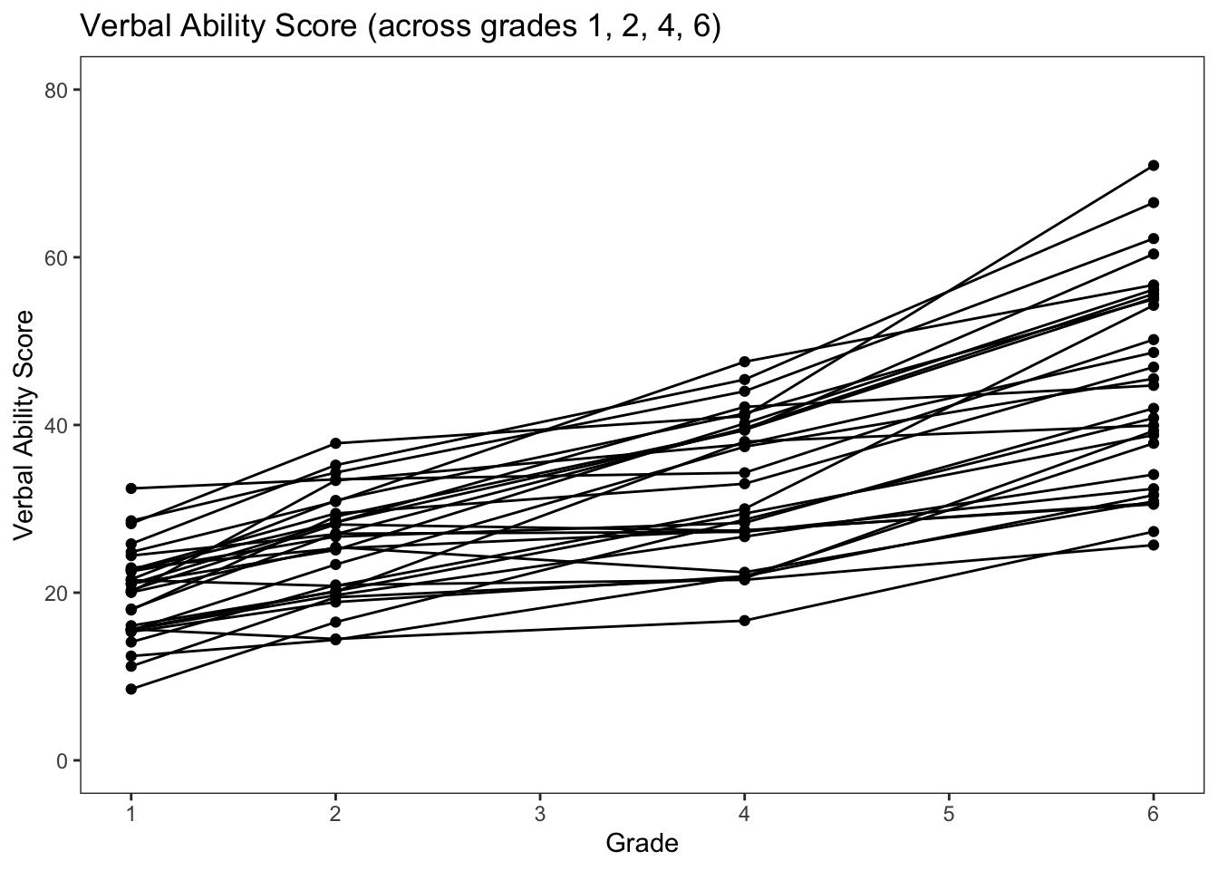
Sometimes the “blob” gets too dense. This can be fixed by selecting a subset of persons to visualize.
ggplot(subset(wisclong, id < 30), aes(x = grade, y = verb, group = id)) +
  geom_point() +
  geom_line() +
  scale_x_continuous(breaks=seq(1,6,by=1)) +
  ylim(0,80) +
  ggtitle("Verbal Ability Score (across grades 1, 2, 4, 6)") +
  xlab("Grade") +
  ylab("Verbal Ability Score") +
  theme_bw() +
  theme(
    panel.grid.major = element_blank(),
    panel.grid.minor = element_blank(),
    strip.background = element_blank()
  )
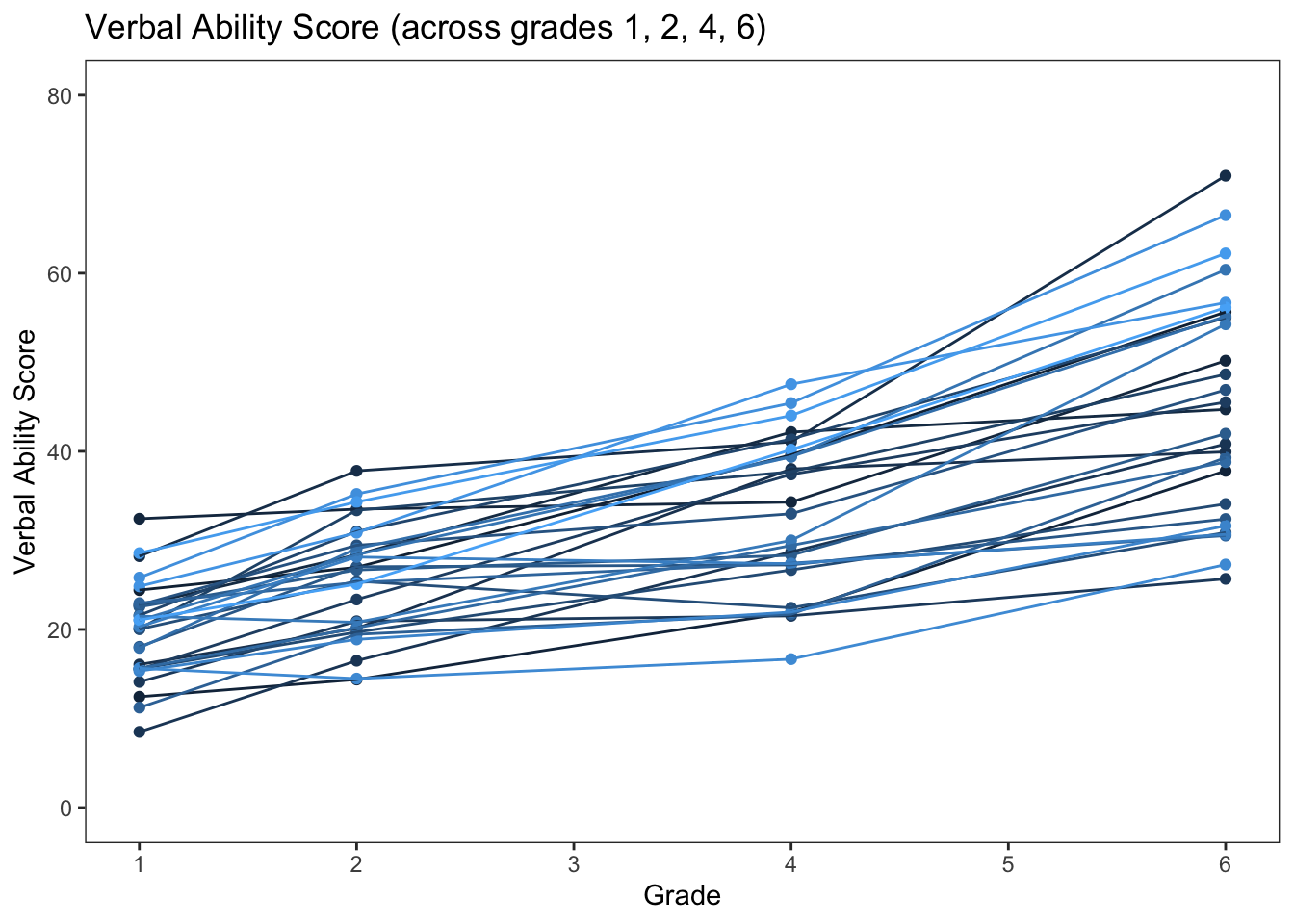
We can add some color to our plot using the color argument and treating id as a factor.
ggplot(subset(wisclong, id < 30), aes(x = grade, y = verb, group = id, color = factor(id))) +
  geom_point() +
  geom_line() +
  scale_x_continuous(breaks=seq(1,6,by=1)) +
  ylim(0,80) +
  ggtitle("Verbal Ability Score (across grades 1, 2, 4, 6)") +
  xlab("Grade") +
  ylab("Verbal Ability Score") +
  theme_bw() +
  theme(
    panel.grid.major = element_blank(),
    panel.grid.minor = element_blank(),
    strip.background = element_blank(),
    legend.position = "none"
  )
We can also get a gradient of colors by treatingid as continuous.
ggplot(subset(wisclong, id < 30), aes(x = grade, y = verb, group = id, color = id)) +
  geom_point() +
  geom_line() +
  scale_x_continuous(breaks=seq(1,6,by=1)) +
  ylim(0,80) +
  ggtitle("Verbal Ability Score (across grades 1, 2, 4, 6)") +
  xlab("Grade") +
  ylab("Verbal Ability Score") +
  theme_bw() +
  theme(
    panel.grid.major = element_blank(),
    panel.grid.minor = element_blank(),
    strip.background = element_blank(),
    legend.position = "none"
  )
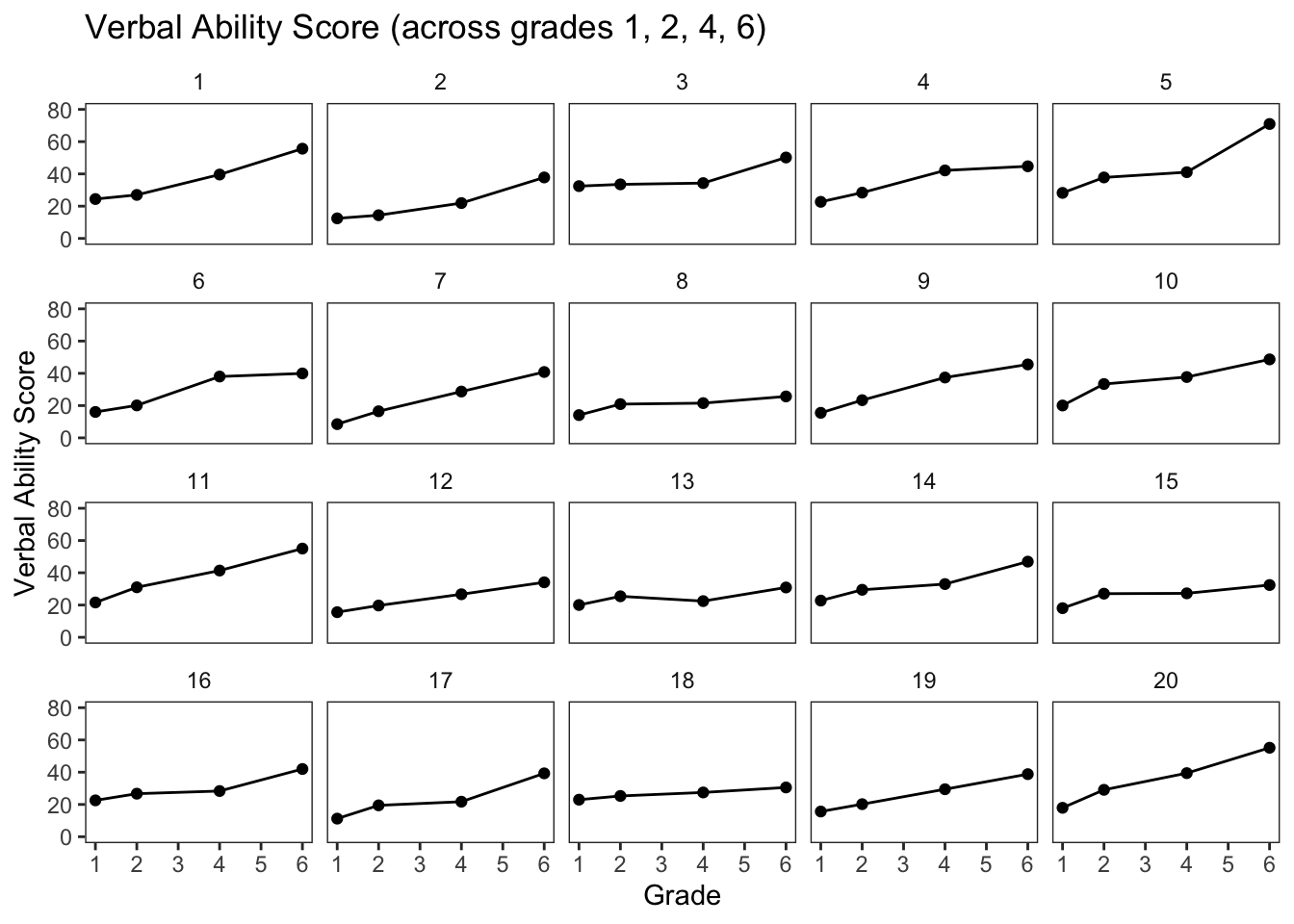
It is also sometimes useful to look at the collection of individual-level plots.
ggplot(subset(wisclong, id <= 20), aes(x = grade, y = verb)) +
  geom_point() +
  geom_line() +
  scale_x_continuous(breaks=seq(1,6,by=1)) +
  ylim(0,80) +
  ggtitle("Verbal Ability Score (across grades 1, 2, 4, 6)") +
  xlab("Grade") +
  ylab("Verbal Ability Score") +
  theme_bw() +
  facet_wrap( ~ id) +
  theme(
    panel.grid.major = element_blank(),
    panel.grid.minor = element_blank(),
    strip.background = element_blank(),
    legend.position = "none"
  )
Some other aesthetics to get to the formal APA style.
#ggplot version .. see also http://ggplot.yhathq.com/docs/index.html
ggplot(subset(wisclong, id <= 20), aes(x = grade, y = verb, group = id)) +
  geom_point() +
  geom_line() +
  xlab("Grade") +
  ylab("WISC Verbal Score") +
  ylim(0,100) +
  scale_x_continuous(breaks=seq(1,6,by=1)) +
  ggtitle("Intraindividual Change in Verbal Ability") +
  theme_classic() +
  #increase font size of axis and point labels
  theme(axis.title = element_text(size = rel(1.5)),
        axis.text = element_text(size = rel(1.2)),
        legend.position = "none")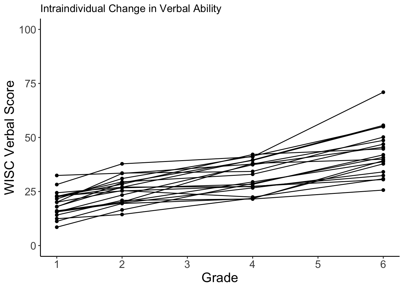
Saving the plot file. See also outputting plots to a file.
Now we have a good set of strategies to apply when looking at new longitudinal data.