14.3 Example Data (Ram & Grimm, 2007)
This chapter’s exercises are based on a script from Drs. Nilam Ram and Kevin Grimm, which was made for the purpose of illustrating the analyses that were done in their paper (Ram and Grimm 2007).
This script includes the cortisol data for \(34\) subjects across \(9\) timepoints (\(N = 34, T = 9\)) collected over the course of a few hours. The experimental design consisted of three phases used to inestigate the time-course of cortisol production and dispersion in response to a controlled intervention:
- Baseline: \(t=0,1\)
- Intervention (driving simulator): \(t=2,3,4\)
- Post-Intervention Follow-up: \(t=5,6,7,8\)
This data set has been used to illustrate a variety of growth modeling and mixture modeling methods (Grimm et al. 2013; Ram and Grimm 2009). We describe the data and then walk through R-based implementations of the models covered in
Ram, N., & Grimm, K. (2007). Using simple and complex growth models to articulate developmental change: Matching theory to method. International Journal of Behavioral Development, 31, 303-316.
The data are shared with intent that others may find them useful for learning about growth modeling or developing new methods for analysis of change. New publications based on these data require citation and acknowledgement of the full set of papers that have used the data, including the above papers.
Thanks are also given to John Nesselroade, Teresa Seeman, and Marilyn Albert for data collection and inspiration.
14.3.1 Read in Cortisol Data
library(psych)
library(ggplot2)
library(nlme)
library(lme4)

filepath <- "https://quantdev.ssri.psu.edu/sites/qdev/files/TheCortisolData.csv"
cortisol_wide <- read.csv(file=url(filepath),header=TRUE)
head(cortisol_wide,6)
## id cort_0 cort_1 cort_2 cort_3 cort_4 cort_5 cort_6 cort_7 cort_8
## 1 1 4.2 4.1 9.7 14.0 19.0 18.0 20.0 23.0 24.0
## 2 2 5.5 5.6 14.0 16.0 19.0 17.0 18.0 20.0 19.0
## 3 3 4.0 3.8 7.5 12.0 14.0 13.0 9.1 8.2 7.9
## 4 4 6.1 5.6 14.0 20.0 26.0 23.0 26.0 25.0 26.0
## 5 5 4.6 4.4 7.2 12.3 15.8 16.1 17.0 17.8 19.1
## 6 6 6.8 9.5 14.2 19.6 19.0 13.9 13.4 12.5 11.714.3.2 Reshaping Data
We already have the wide format data. We make a set of long format data.
cortisol_long <- reshape(
  data = cortisol_wide,
  timevar = c("time"),
  idvar = "id",
  varying = c("cort_0","cort_1","cort_2",
              "cort_3","cort_4","cort_5",
              "cort_6","cort_7","cort_8"),
  direction="long",
  sep="_"
)
# sorting for easy viewing  order by id and time
cortisol_long <- cortisol_long[order(cortisol_long$id,cortisol_long$time), ]
To match the scaling of time used in some of the papers we add an additional time variable that runs from 0 to 1.
Looking at the top few rows of the long data.
##     id time cort timescaled
## 1.0  1    0  4.2      0.000
## 1.1  1    1  4.1      0.125
## 1.2  1    2  9.7      0.250
## 1.3  1    3 14.0      0.375
## 1.4  1    4 19.0      0.500
## 1.5  1    5 18.0      0.625
## 1.6  1    6 20.0      0.750
## 1.7  1    7 23.0      0.875
## 1.8  1    8 24.0      1.000
## 2.0  2    0  5.5      0.000
## 2.1  2    1  5.6      0.125
## 2.2  2    2 14.0      0.250
## 2.3  2    3 16.0      0.375
## 2.4  2    4 19.0      0.500
## 2.5  2    5 17.0      0.625
## 2.6  2    6 18.0      0.750
## 2.7  2    7 20.0      0.875
## 2.8  2    8 19.0      1.000
14.3.3 Descriptives
Basic descriptives of the 9-occasion data.
##        vars  n  mean   sd median trimmed   mad min  max range  skew kurtosis
## id        1 34 17.50 9.96  17.50   17.50 12.60   1 34.0  33.0  0.00    -1.31
## cort_0    2 34  5.25 2.45   5.00    4.90  2.30   2 12.0  10.0  1.18     0.92
## cort_1    3 34  5.06 2.59   4.50    4.78  2.22   2 11.3   9.3  1.02    -0.01
## cort_2    4 34 10.85 3.11  10.05   10.79  3.85   6 16.7  10.7  0.09    -1.17
## cort_3    5 34 17.36 3.69  17.35   17.39  3.48   7 24.9  17.9 -0.29     0.39
## cort_4    6 34 19.48 3.72  19.10   19.49  2.82  12 27.1  15.1 -0.04    -0.56
## cort_5    7 34 16.46 4.18  16.95   16.41  4.52   8 26.0  18.0  0.08    -0.58
## cort_6    8 34 15.03 4.57  14.65   14.90  4.15   6 26.0  20.0  0.26    -0.31
## cort_7    9 34 15.62 4.81  16.15   15.60  5.56   7 25.0  18.0 -0.02    -0.99
## cort_8   10 34 15.86 5.61  16.00   15.81  6.08   6 26.0  20.0  0.14    -1.08
##          se
## id     1.71
## cort_0 0.42
## cort_1 0.44
## cort_2 0.53
## cort_3 0.63
## cort_4 0.64
## cort_5 0.72
## cort_6 0.78
## cort_7 0.82
## cort_8 0.96
#boxplot by day
ggplot(data=cortisol_long, aes(x=factor(time), y=cort)) +
geom_boxplot(notch = TRUE) +
stat_summary(fun.y="mean", geom="point", shape=23, size=3, fill="white") +
labs(x = "Time", y = "Cortisol") +
theme_classic()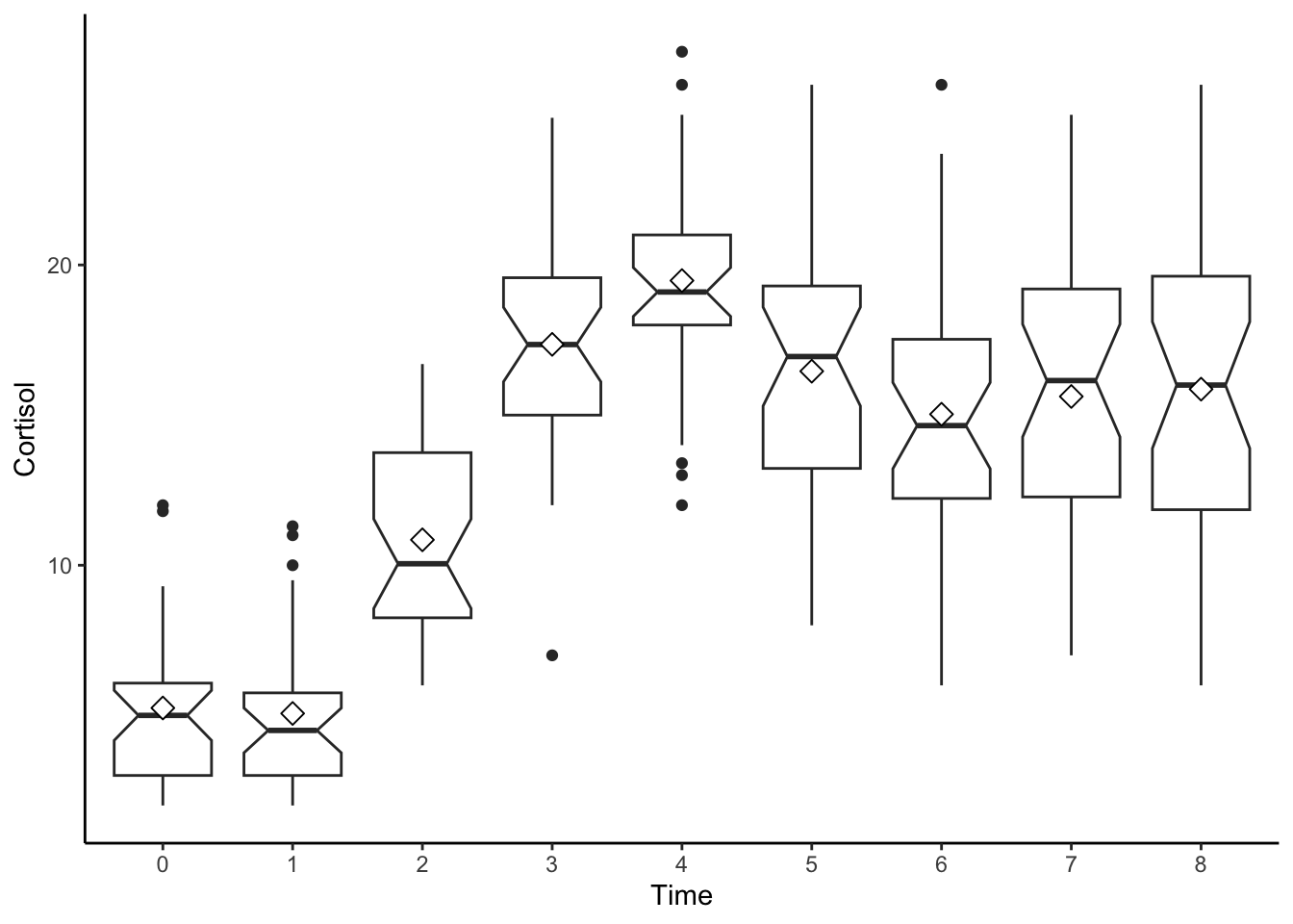
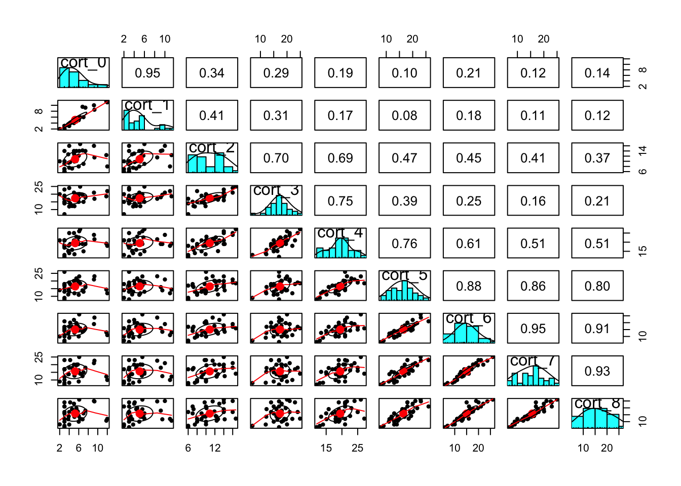
#pairs plot from the psych library
psych::pairs.panels(
  cortisol_wide[,c(
    "cort_0","cort_1","cort_2",
    "cort_3","cort_4","cort_5",
    "cort_6","cort_7","cort_8"
),])
14.3.4 Density Plots
#Density distribution by day
ggplot(data=cortisol_long, aes(x=cort)) +
  geom_density(aes(group=factor(time), colour=factor(time), fill=factor(time)), alpha=0.3) +
  theme_classic()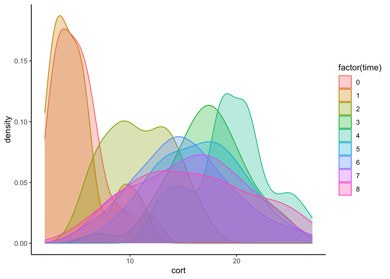
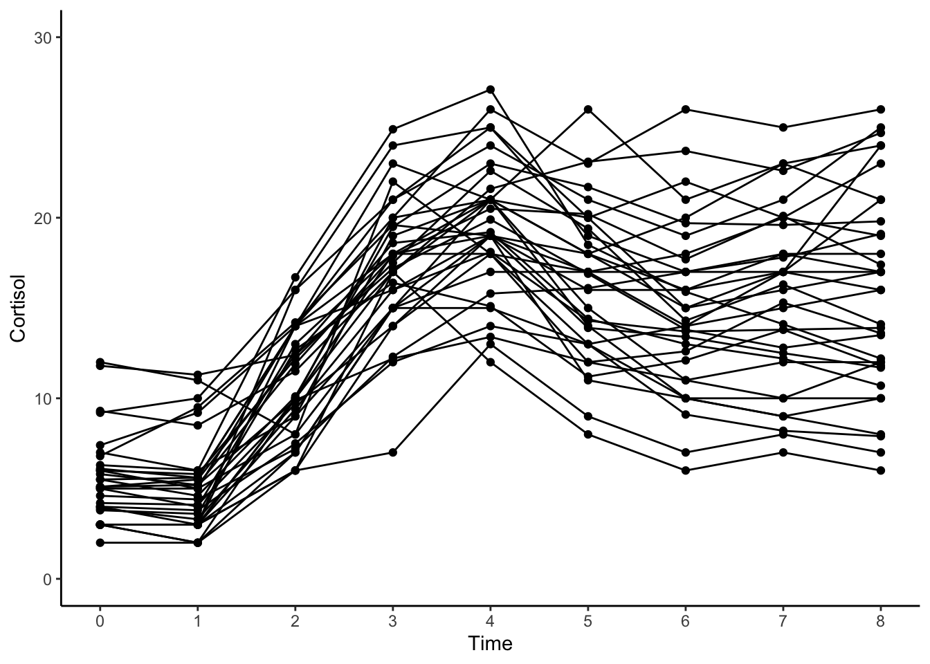
14.3.5 Individual-level Trajectories
#intraindividual change trajetories
ggplot(data = cortisol_long, aes(x = time, y = cort, group = id)) +
  geom_point(color="black") +
  geom_line(color="black") +
  xlab("Time") +
  ylab("Cortisol") + ylim(0,30) +
  scale_x_continuous(breaks=seq(0,8,by=1)) +
  theme_classic()