17.2 The N=1 AR Model
First, let’s consider the most simple time-series model. Here we only show 4 timepoints, typically the time series will be considerably longer.
17.2.1 Random Shocks
First, let’s consider the random shock \(z_t, t=1,\dots,T\).
These random shocks have a number of interesting properties.
- Random shocks are latent variables.
- Random shocks are identically distributed with variance \(\psi\), e.g., \(z_t \sim \mathcal{N}(0,\psi)\).
- A shock at any time point influences the process variable at two or more time points.
- Intuitively, shocks represent all the unmodeled influences that effect the process variable.
- Shock are the dynamic part of the time series model.
- Random shocks perturb the system and change its course over time.
- Although errors, random shocks differ from measurement errors in meaningful ways.
- Random shocks differ from other errors in that they influence the process variable at more than 1 time point.
17.2.2 Autoregressive Parameter
Next, let’s consider the autorgressive coefficient \(\alpha_1\). In an AR(1) model, where only one lag is considered, the AR coefficients are generally the parameter of interest.
The interest in an individual’s autoregressive parameter stems from the fact that this parameter indexes the time it takes an individual to recover from a random shock and return to equilibrium.
- An AR close to zero implies that there is little carryover from one measurement occasion to the next and recovery is thus instant.
- An AR parameter close to one implies that there is considerable carryover between consecutive measurement occasions, such that perturbations continue to have an effect on subsequent occasions.
- AR parameters can be interpreted as a measure of inertia, stability or regulatory weakness.
Positive and Negative AR Parameters
- A positive AR parameter could be expected for many psychological processes, such as that of mood, attitudes symptoms.
- A negative alpha indicates that if an individual has a high score at one occasion, the score at the next occasion is likely to be low, and vice versa.
17.2.3 AR(1) Model Example
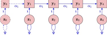
Consider a simple AR(1) model,
\[ y_{t} = \alpha_{1}y_{t-1} + z_{t}\nonumber \] which matches the path diagram:
Looking at the path diagram above, suppose
- \(y_{t}\) are hourly measurements of concentration.
- \(z_t\) Unobserved events impacting concentration.
Here we might imagine that during one of these intervals the subject gets some bad news. This might result in a decreased concentration levels at that measurement occasion, and this effect effect may then linger for the next few measurement occasions (as a result of an AR effect). The larger the AR coefficient, the longer it will take for the student to return to their baseline concentration level.
Discussion Question:
Choose a single variable (or construct) from your own research.
- How would you measure this variable across time (e.g. self-report via mobile phone)?
- How often would you measure the variable to capture important fluctuations?
- If you fit a simple AR(1) model to the repeated measures how might you interpret the autoregressive effect?
17.2.4 Fitting a AR(1) Model in R
Let’s load the libraries we’ll need for this chapter.
## Loading required package: httr## Warning: package 'mlVAR' was built under R version 4.3.2Consider some example data from the Many Analysts project: https://osf.io/h3djy/
The experience sampling methodology (ESM) has been positioned as a promising opportunity for personalized medicine in psychiatry. A requisite for moving ESM towards clinical practice is that outcomes of person-centered analyses are not contingent on the researcher. In this study, we crowdsourced the analysis of one individual patient’s ESM data to 12 prominent research teams to investigate how much researchers vary in their analytical approach towards individual time series data and to what degree outcomes vary based on analytical choices.
This is a description of the project taken from https://osf.io/wfzr7/:
Research question:
What symptom(s) would you advise the treating clinician to target subsequent treatment on, based on a person-centered analysis of this particular patient’s EMA data? To answer this research question, please analyze the dataset in whatever manner your research team sees as best.
The Dataset:
The data used in this project stem from the research lab of Aaron Fisher (UC Berkeley).
From this dataset one subject was chosen for the current project. The data were saved as a csv file (comma delimited). Selection of the dataset was based on the following criteria: the subject has a primary diagnosis of major depressive disorder (MDD), the dataset includes more than 100 time points, and the dataset has some missingness.
The subject (ID 3) was a white 25-year old male with a primary diagnosis of MDD and a comorbid generalized anxiety disorder (GAD). His Hamilton Rating Scale for Depression score was 16 and his Hamilton Rating Scale for Anxiety score was 15.
In the experiment by Fisher, subjects were asked to fill out a survey on their mobile phones 4 times a day for 30 days. Surveys were conducted at a random time within each of four 3-hourblocks, with the additional constraint that surveys should be given at least 30 minutes apart. At each sampling occasion, subjects were prompted to think about the period of time since the last survey. Items were scored on a visual analogue slider ranging from 0 to 100 with the endpoints “not at all” and “as much as possible”.
Variables in Dataset
- energetic (felt energetic)
- enthusiastic (felt enthusiastic)
- content (felt content)
- irritable (felt irritable)
- restless (felt restless)
- worried (felt worried)
- guilty (felt worthless or guilty)
- afraid (felt frightened or afraid)
- anhedonia (felt a loss of interest or pleasure)
- angry (felt angry)
- hopeless (felt hopeless)
- down (felt down or depressed)
- positive (felt positive)
- fatigue (felt fatigued)
- tension (experienced muscle tension)
- concentrate (experienced difficulty concentrating)
- accepted (felt accepted or supported)
- threatened (felt threatened, judged, or intimidated)
- ruminate (dwelled on the past)
- avoid_act (avoided activities)
- reassure (sought reassurance)
- procrast (procrastinated)
- hours (how many hours did you sleep last night?)
- difficult (experienced difficulty falling or staying asleep)
- unsatisfy (experienced restless or unsatisfying sleep)
- avoid_people (avoided people)
Let’s read in the data:
url <- 'https://osf.io/tcnpd//?action=download'
filename <- 'osf_dataframe.csv'
GET(url, write_disk(filename, overwrite = TRUE))
## Response [https://files.osf.io/v1/resources/b7ar3/providers/osfstorage/592ff0d39ad5a1026250f506?action=download&direct&version=1]
## Date: 2024-04-15 14:25
## Status: 200
## Content-Type: text/csv
## Size: 25.8 kB
## <ON DISK> /Users/zff100/Dropbox/Macbook/PSU/Courses/HDFS523/ZZ_bookdown/HDFS523-master/HDFS523/osf_dataframe.csv## X start finish energetic enthusiastic content irritable
## 1 1 10/28/2014 17:15 10/28/2014 17:19 34 28 34 73
## 2 2 10/28/2014 21:30 10/28/2014 21:56 50 26 31 70
## 3 3 10/29/2014 9:22 10/29/2014 10:02 32 32 35 63
## 4 4 10/29/2014 13:41 10/29/2014 13:45 45 24 26 63
## 5 5 10/29/2014 17:40 10/29/2014 17:42 27 24 21 60
## 6 6 10/29/2014 21:54 10/29/2014 22:18 35 16 41 32
## restless worried guilty afraid anhedonia angry hopeless down positive fatigue
## 1 60 68 59 34 39 61 63 66 36 62
## 2 60 64 65 60 34 57 64 78 33 50
## 3 56 58 34 56 35 63 64 62 40 36
## 4 66 65 24 29 31 58 65 60 35 39
## 5 61 64 31 24 45 45 48 60 38 71
## 6 27 65 51 31 27 26 43 47 42 47
## tension concentrate accepted threatened ruminate avoid_act reassure procrast
## 1 61 33 42 59 84 29 38 24
## 2 58 31 48 47 90 39 61 34
## 3 56 30 54 37 60 44 44 36
## 4 67 33 37 27 79 17 40 17
## 5 53 34 50 29 61 31 40 35
## 6 57 22 43 15 78 14 32 27
## hours difficult unsatisfy avoid_people NA. NA..1 NA..2
## 1 8.0 41 28 20 <NA> 0.000000 0.00000
## 2 NA NA NA 34 10/28/2014 17:15 4.250000 4.25000
## 3 5.5 63 67 22 10/28/2014 21:30 11.866667 16.11667
## 4 NA NA NA 18 10/29/2014 9:22 4.316667 20.43333
## 5 NA NA NA 35 10/29/2014 13:41 3.983333 24.41667
## 6 NA NA NA 20 10/29/2014 17:40 4.233333 28.65000
## lag tdif cumsumT
## 1 <NA> 0.000000 0.00000
## 2 10/28/2014 17:15 4.250000 4.25000
## 3 10/28/2014 21:30 11.866667 16.11667
## 4 10/29/2014 9:22 4.316667 20.43333
## 5 10/29/2014 13:41 3.983333 24.41667
## 6 10/29/2014 17:40 4.233333 28.65000Now, let’s use the concentrate variable.
The first step in an autoregressive analysis typically involves lagging the data. We can do this for a single-la as follows:
first           <- df[1:(nrow(df)-1), ]
second          <- df[2:(nrow(df)  ), ]
lagged_df       <- data.frame(first, second)
colnames(lagged_df) <- c(paste0(colnames(df), "lag"), colnames(df))
head(lagged_df)
## concentratelag concentrate
## 1 33 31
## 2 31 30
## 3 30 33
## 4 33 34
## 5 34 22
## 6 22 27Now, with our data lagged we can fit an AR model using OLS as follows:
##
## Call:
## lm(formula = concentrate ~ concentratelag, data = lagged_df)
##
## Residuals:
##     Min      1Q  Median      3Q     Max
## -22.279 -13.082  -5.119  12.611  48.776
##
## Coefficients:
##                Estimate Std. Error t value Pr(>|t|)
## (Intercept)    36.84675    4.07468   9.043 1.07e-14 ***
## concentratelag  0.01885    0.09903   0.190    0.849
## ---
## Signif. codes:  0 '***' 0.001 '**' 0.01 '*' 0.05 '.' 0.1 ' ' 1
##
## Residual standard error: 16.59 on 102 degrees of freedom
##   (17 observations deleted due to missingness)
## Multiple R-squared:  0.000355,   Adjusted R-squared:  -0.009445
## F-statistic: 0.03622 on 1 and 102 DF,  p-value: 0.8494
17.2.5 AR Coefficients Example
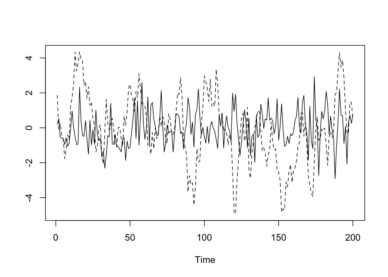
Let’s consider what a time series looks like when it is generated with different AR values.
The time series with an autoregressive coefficient of \(0.1\) is the solid black line. The time series with an autoregressive coefficient of \(0.9\) is the dashed line.
set.seed(1234)
y1 <- arima.sim(list(order=c(1,0,0), ar=.1), n=200)
y2 <- arima.sim(list(order=c(1,0,0), ar=.9), n=200)
ts.plot(y1,y2,lty=c(1:2))