9.7 Revisisting Overdispersion

Let’s run our model fit test based on the deviance for model2.

1 - pchisq(summary(model2)$deviance, summary(model2)$df.residual )

## [1] 0

Again, we reject the hypothesis of a close fit between model and data. To gain a little more insight we can plot estimates of the variance against the expected value, alongside a line with an intercept of zero and a slope of 1.

We expect the data points to fall somewhat evenly along that line. Here, it appears our variance is consistently larger than our mean, indicating the possibility of overdispersion.

plot(
  log(fitted(model2)),
  log((ferraro2016$morbidityw1-fitted(model2))^2),
  xlab=expression(hat(mu)),
  ylab=expression((y-hat(mu))^2),
  pch=20,col="blue"
)
abline(0,1) ## 'varianc = mean' line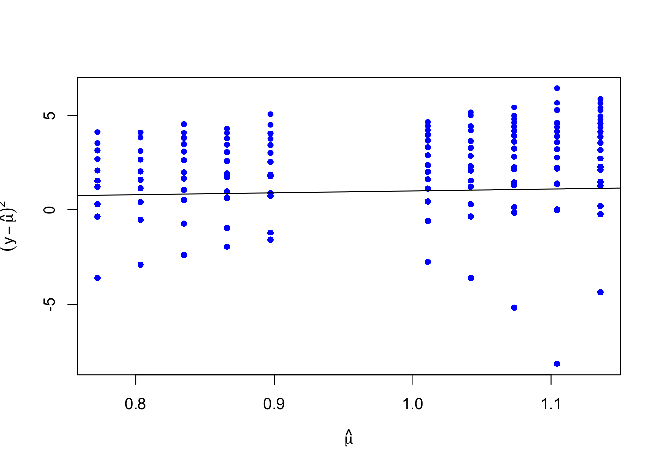

We can also run some formal tests for overdispersion. For example, using the AER package we can estimate an overdispersion parameter and test whether or not it equals zero.

AER::dispersiontest(model2,trafo=1)

## Warning in y - yhat: longer object length is not a multiple of shorter object
## length

## Warning in (y - yhat)^2 - y: longer object length is not a multiple of shorter
## object length

## 
##  Overdispersion test
## 
## data:  model2
## z = 13.22, p-value < 2.2e-16
## alternative hypothesis: true alpha is greater than 0
## sample estimates:
##    alpha 
## 1.986701

Here we clearly see that there is evidence of overdispersion (\(\alpha\) is estimated to be 1.986) which speaks quite strongly against the assumption of equidispersion (i.e. \(\alpha=0\)).

One way to handle this is to fit a estimate with overdispersion parameter directly in the model using a quassipoison approach.

9.7.1 Quassi-Poisson Family

If we want to test and adjust for overdispersion we can add a scale parameter with the family=quasipoisson option. The estimated scale parameter will be labeled as Overdispersion parameter in the output.

model3 <- glm(
  formula = morbidityw1 ~ 1 + abuse_rare + income_star + abuse_rare:income_star, 
  family = quasipoisson(link=log), 
  data = ferraro2016,
  na.action = na.exclude
)
summary(model3)

## 
## Call:
## glm(formula = morbidityw1 ~ 1 + abuse_rare + income_star + abuse_rare:income_star, 
##     family = quasipoisson(link = log), data = ferraro2016, na.action = na.exclude)
## 
## Coefficients:
##                           Estimate Std. Error t value Pr(>|t|)    
## (Intercept)              1.0766511  0.0217425  49.518  < 2e-16 ***
## abuse_rare1             -0.2382614  0.0421387  -5.654 1.71e-08 ***
## income_star             -0.0311089  0.0153759  -2.023   0.0431 *  
## abuse_rare1:income_star -0.0000822  0.0300781  -0.003   0.9978    
## ---
## Signif. codes:  0 '***' 0.001 '**' 0.01 '*' 0.05 '.' 0.1 ' ' 1
## 
## (Dispersion parameter for quasipoisson family taken to be 2.812535)
## 
##     Null deviance: 8068.4  on 2966  degrees of freedom
## Residual deviance: 7956.7  on 2963  degrees of freedom
##   (55 observations deleted due to missingness)
## AIC: NA
## 
## Number of Fisher Scoring iterations: 5

The new standard errors (in comparison to the model without the overdispersion parameter), are larger, Thus, the Wald statistics will be smaller and less likely to be significant.

We could also use a likelihood-ratio test to test whether a quasipoisson GLM with overdispersion is significantly better than a regular poisson GLM without overdispersion :

pchisq(summary(model3)$dispersion * model2$df.residual, 
               model2$df.residual, lower = FALSE)

## [1] 0

This results suggest we would reject the null hypothesis of the Poisson regression being a superior fit to the quasipoisson approach, providing evidence for the quasipoisson model.

9.7.2 Marginal Effects Examples

Fit our main model.

model4 <- glm(
  formula = morbidityw1 ~ 1 + health + abuse_rare + income_star + abuse_rare:income_star, 
  family = quasipoisson(link=log), 
  data = ferraro2016,
  na.action = na.exclude
)
summary(model4)

## 
## Call:
## glm(formula = morbidityw1 ~ 1 + health + abuse_rare + income_star + 
##     abuse_rare:income_star, family = quasipoisson(link = log), 
##     data = ferraro2016, na.action = na.exclude)
## 
## Coefficients:
##                           Estimate Std. Error t value Pr(>|t|)    
## (Intercept)              9.959e-01  2.883e-02  34.541  < 2e-16 ***
## health                   1.855e-01  4.209e-02   4.406 1.09e-05 ***
## abuse_rare1             -2.215e-01  4.201e-02  -5.273 1.43e-07 ***
## income_star             -2.637e-02  1.529e-02  -1.724   0.0848 .  
## abuse_rare1:income_star  7.307e-05  2.984e-02   0.002   0.9980    
## ---
## Signif. codes:  0 '***' 0.001 '**' 0.01 '*' 0.05 '.' 0.1 ' ' 1
## 
## (Dispersion parameter for quasipoisson family taken to be 2.769737)
## 
##     Null deviance: 8068.4  on 2966  degrees of freedom
## Residual deviance: 7904.2  on 2962  degrees of freedom
##   (55 observations deleted due to missingness)
## AIC: NA
## 
## Number of Fisher Scoring iterations: 5

In GLM models, most quantities of interest are conditional, in the sense that they will typically depend on the values of all the predictors in the model. Therefore, we need to decide where in the predictor space we want to evaluate the quantity of interest described above.