4.2 Operations on Matrices
4.2.1 Matrix Transpose
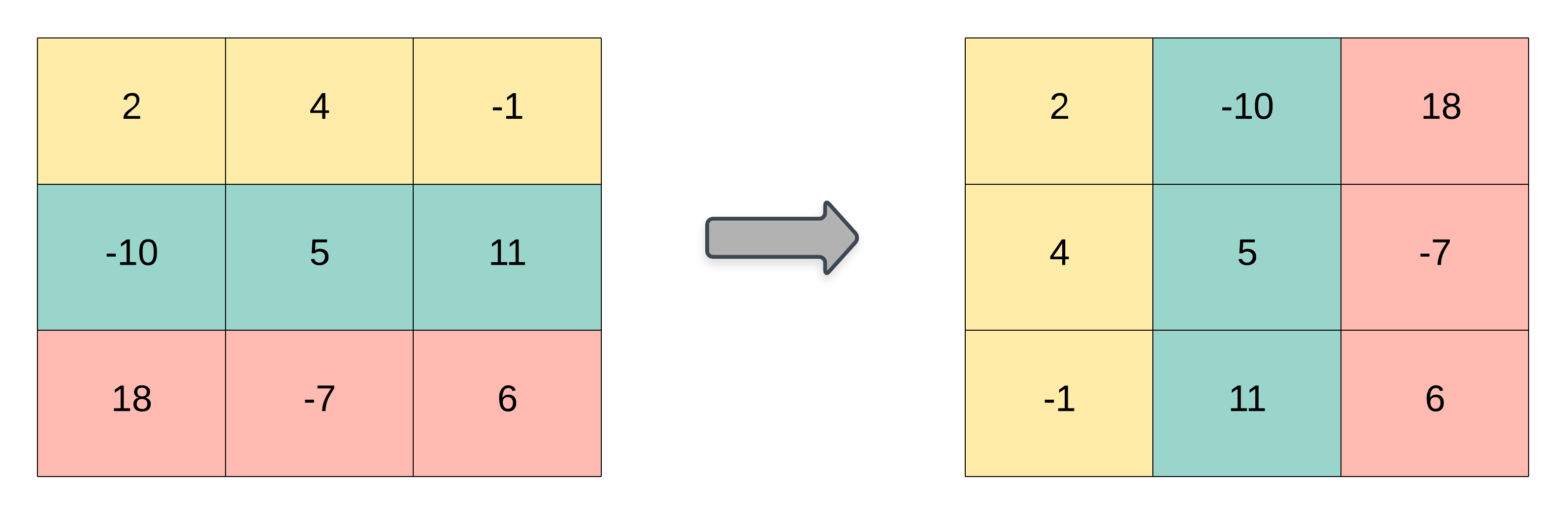
As stated earlier the transpose of a matrix is an operator which flips a matrix over its diagonal. That is, it switches the row and column indices of the matrix \(A\) by producing another matrix, often denoted by \(A'\) (or \(A^{T}\)). Some useful properties of the matrix transpose include:
\[ (\mathbf{A + B})' = \mathbf{A' + B'}\\ (c\mathbf{A'}) = c(\mathbf{A'}) = (\mathbf{A'})c \\ (\mathbf{A'B}) = \mathbf{B'A}\\ (\mathbf{AB})' = \mathbf{B'A'}\\ (\mathbf{A'})' = \mathbf{A} \] Graphical Depiction of a Matrix Transpose
4.2.2 Matrix Trace
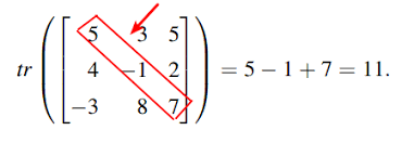
The trace of a square matrix is the sum of elements along the diagonal. The trace is only defined for a square matrix. For an \(n \times n\) matrix the trace is defined as follows:
\[ tr(\mathbf{A}) = \sum_{i=1}^{n}{a_{ii}} = a_{11} + a_{22} + ... + a_{nn} \] Graphical Depiction of a Matrix Trace
Some useful properties of the matrix trace include:
\[ tr(\mathbf{A + B}) = tr(\mathbf{A}) + tr(\mathbf{B})\\ tr(c\mathbf{A}) = c(tr(\mathbf{A})) \\ tr(\mathbf{A}) = tr(\mathbf{A'})\\ tr(\mathbf{AB}) = tr(\mathbf{BA})\\ tr(\mathbf{ABC}) = tr(\mathbf{CAB})=tr(\mathbf{BCA}) \]
4.2.3 Addition
For addition, matrices must be of the same order. Addition of two matrices is accomplished by adding corresponding elements, \(c_{ij}=a_{ij}+b_{ij}\)
\[ \mathbf{A} = \begin{bmatrix} 10 & 5 \\ 9 & 1 \end{bmatrix} , \enspace \mathbf{B} = \begin{bmatrix} 2 & 1 \\ 20 & 0 \end{bmatrix}, \enspace \textrm{then } \mathbf{A}+\mathbf{B}= \begin{bmatrix} 12 & 6 \\ 29 & 1 \end{bmatrix} \] Matrix addition is commutative (gives the same result whatever the order of the quantities involved),
\[ \mathbf{A + B} = \mathbf{B + A} \] and associative (gives the same result whatever grouping their is, as long as order remains the same),
\[ \mathbf{A + (B + C)} = \mathbf{(A + B) + C} \] and
\[ \mathbf{A + (-B)} = \mathbf{(A - B)}. \]
4.2.4 Subtraction
Like addition, subtraction requires matrices of the same order. Elements in the difference matrix are given by the algebraic difference between corresponding elements in matrices being subtracted:
\[ \mathbf{A} = \begin{bmatrix} 10 & 5 \\ 9 & 1 \end{bmatrix} , \enspace \mathbf{B} = \begin{bmatrix} 2 & 1 \\ 20 & 0 \end{bmatrix}, \enspace \textrm{then } \mathbf{A}-\mathbf{B}= \begin{bmatrix} 8 & 4 \\ -11 & 1 \end{bmatrix} \]
4.2.5 Matrix Multiplication
Three useful rules to keep in mind regarding matrix multiplication:
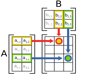
Only matrices of the form \((m \times n) * (n \times p)\) are conformable for multiplication. The number of columns in the premultiplier must equal the number of rows in the post multiplier.
The product matrix will have the following order: \(\mathbf{A}_{m\times n} \mathbf{B}_{n\times p} = \mathbf{C}_{m \times p}\).
Graphical Depiction of Rules 1 and 2

- The element \(c_{ij}\) in the product matrix is the result of multiplying row \(i\) of the premultiplier matrix, and row \(j\) of the post multiplier matrix (e.g. (\(c_{ij}=a_{i1}b_{1j} + a_{i2}b_{2j} + a_{i3}b_{3j}\))).
Graphical Depiction of Rule 3
Matrix multiplication is associative (i.e. rearranging the parentheses in an expression will not change the result). That is,
\[ \mathbf{(AB)C} = \mathbf{A(BC)} \] and is distributive with respect to addition, \[ \mathbf{A(B+C)} = \mathbf{AB + AC} \\ \mathbf{(B+C)A} = \mathbf{BA + CA} \\ \] If \(c\) is a scalar, then
\[ c(\mathbf{AB})=c(\mathbf{A})\mathbf{B}=\mathbf{A}(c\mathbf{B})=(\mathbf{AB})c \] or equivalently,
\[ \mathbf{A} = \begin{bmatrix} 10 & 5 \\ 9 & 1 \end{bmatrix}, \enspace k=2, \enspace k\mathbf{A} = \begin{bmatrix} 20 & 10 \\ 18 & 2 \end{bmatrix}. \]
In general, matrices that can be multiplied are called ‘compatible’ or ‘comformable.’ Matrices in which the inner dimensions (i.e., columns of \(\mathbf{A}\), rows of \(\mathbf{B}\)) do not match are called ‘incompatible’ or ‘non-conformable.’ These cannot be multiplied.
4.2.6 Matrix Division
Division is not defined for matrix operations, but may be accomplished by multiplication by the inverse matrix. In algebra, the reciprocal of a scalar is, by definition, the scalar raised to the minus one power (e.g. \(5^{-1} = 1/5\)), and equations may be solved by multiplication by reciprocals.
For example:
\[ 5^{-1} = 1/5\\ 5x=35\\ 5^{-1}(5x)=5^{-1}(35)\\ x = 7 \] Now consider the following equation where the vector \(\mathbf{x}\) is unknown,
\[ \mathbf{A}_{p \times p} \mathbf{x}_{p \times 1} = \mathbf{b}_{p \times 1} \] Each element in the column vector \(\mathbf{x}\) is unknown and the solution involves solving a set of simultaneous equations for the unknown element of \(\mathbf{x}\),
\[ a_{11}x_{1} + a_{12}x_{2} + \dots + a_{1p}x_{p} = b1 \\ a_{21}x_{1} + a_{22}x_{2} + \dots + a_{2p}x_{p} = b2 \\ \vdots \\ a_{p1}x_{1} + a_{p2}x_{2} + \dots + a_{pp}x_{p} = bp \]
A solution analogous to the scalar equations above would give the following solution for the elements of the vector \(\mathbf{x}\):
\[ \mathbf{A}_{p \times p} \mathbf{x}_{p \times 1} = \mathbf{b}_{p \times 1} \\ \mathbf{A}^{-1}_{p \times p}\mathbf{A}_{p \times p} \mathbf{x}_{p \times 1} = \mathbf{A}^{-1}_{p \times p}\mathbf{b}_{p \times 1} \\ \mathbf{I}_{p \times p}\mathbf{x}_{p \times 1} = \mathbf{A}^{-1}_{p \times p}\mathbf{b}_{p \times 1} \\ \mathbf{x}_{p \times 1} = \mathbf{A}^{-1}_{p \times p}\mathbf{b}_{p \times 1} \]
The inverse of a matrix must satisfy the following properties:
\[ \mathbf{AA^{-1}} = \mathbf{A^{-1}A} = \mathbf{I} \] where \(I\) is the identity matrix with 1’s along the diagonal and 0’s elsewhere.
So, why is division undefined for matrices. Here is a quick example. Suppose, \(\mathbf{A}\) is a matrix and \(\mathbf{B}\) is the inverse of \(\mathbf{A}\), such that
\[ \mathbf{AB} = \mathbf{BA} = \mathbf{I} \]
Now, let
\[ \mathbf{A} = \begin{bmatrix} 1 & 2 \\ 1 & 2 \end{bmatrix} , \enspace \mathbf{B} = \begin{bmatrix} a & b \\ c & d \end{bmatrix}, \] Then,
\[ \begin{bmatrix} a & b \\ c & d \end{bmatrix} \begin{bmatrix} 1 & 2 \\ 1 & 2 \end{bmatrix} = \begin{bmatrix} 1 & 0\\ 0 & 1 \end{bmatrix}. \]
This means that \(a+b=1\) and \(2a+2b = 0\), which is a contradiction, suggesting A does not have an inverse.