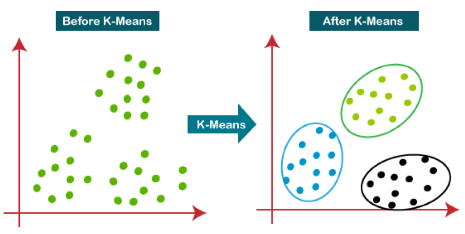
16.5 K-Means Clustering
First specify the desired number of clusters \(K\).
The K-means algorithm will assign each observation to exactly one of the \(K\) clusters.
16.5.1 Within-Cluster Variation
Good clustering is one for which the within-cluster variation is as small as possible The within-cluster variation for cluster \(C_k\) is a measure, \(W(C_k)\), of the amount by which the observations within a cluster differ from each other.
We want to solve
\[ \min_{C_1,\dots,C_{K}} \sum^{K}_{k=1}W(C_{k}) \] Goal is to partition the observations into \(K\) clusters, such that the total within-cluster variation, summed over all \(K\) clusters, is as small as possible.
Let’s define within cluster variation using the squared Euclidian distance (the most commonly used metric)
\[ W(C_{k}) = \frac{1}{|C_k|}\sum_{i,i'\in C_k}\sum_{j=1}^{p}(x_{ij}-x_{i'j})^2 \] Note, clustering with the Euclidean Squared distance metric is faster than clustering with the regular Euclidean distance. Importantly, the output of K-Means clustering is not affected if Euclidean distance is replaced with Euclidean squared distance.
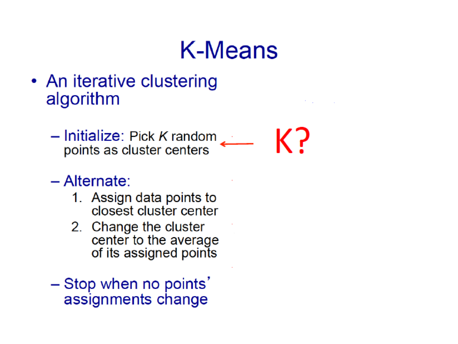
16.5.2 K-Means Algorithm
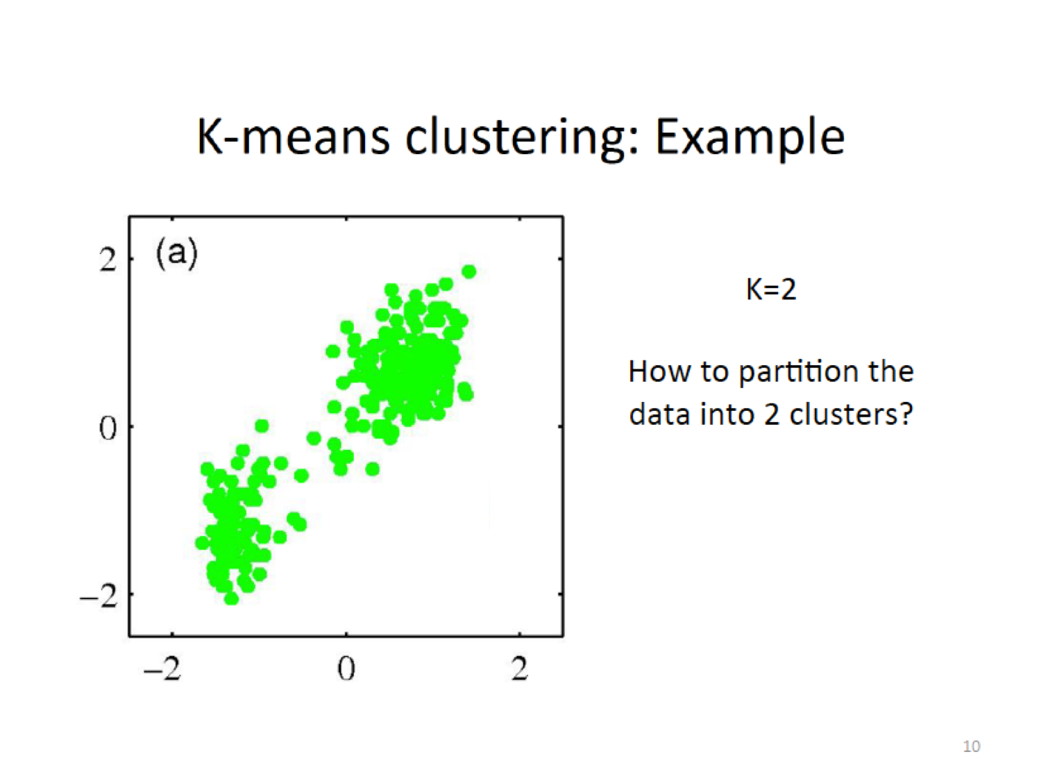
- Specify \(K\), the number of clusters
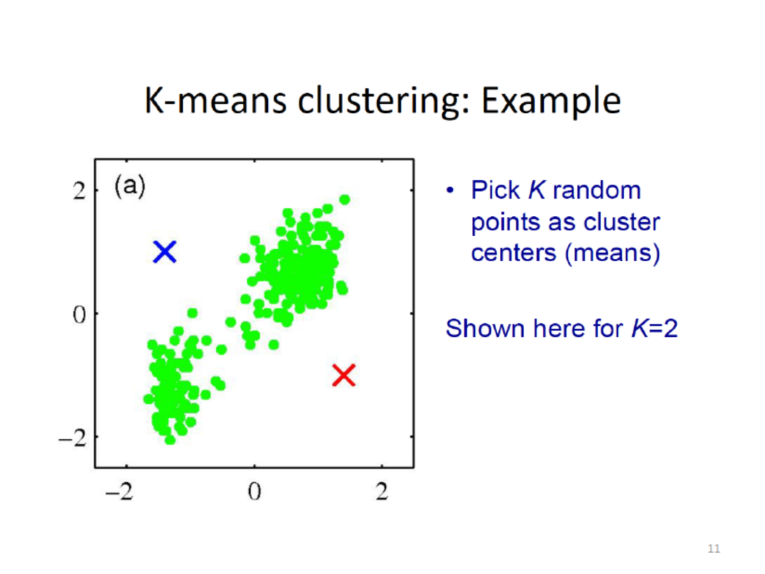
- Randomly select \(K\) initial cluster means (centroids)
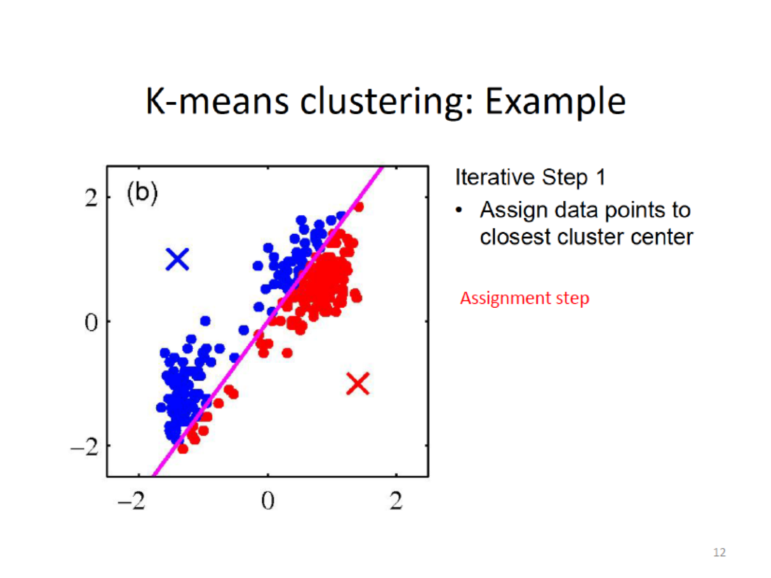
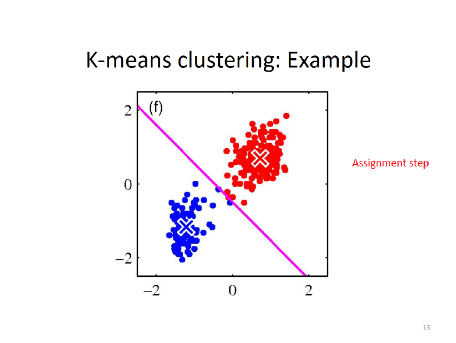
- Assignment step: Assign each observation to the cluster whose centroid is closest (where closest is defined using squared Euclidean distance)
- Adjustment step:Compute the new cluster means (centroids).
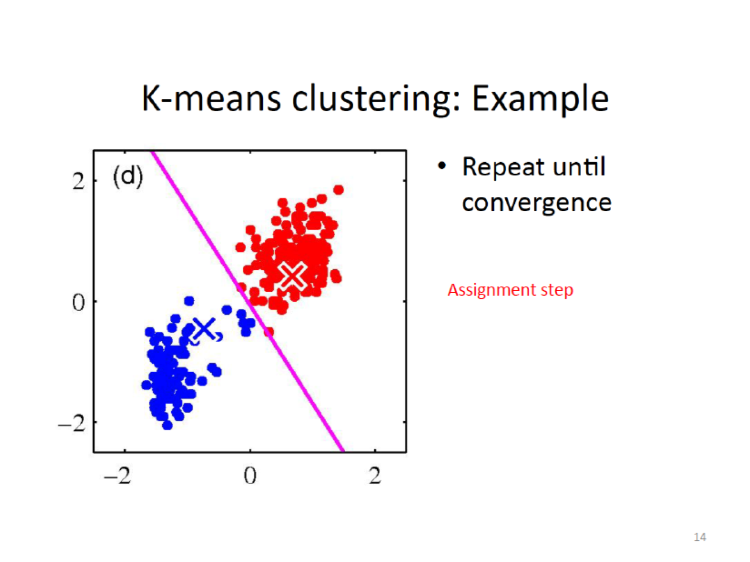
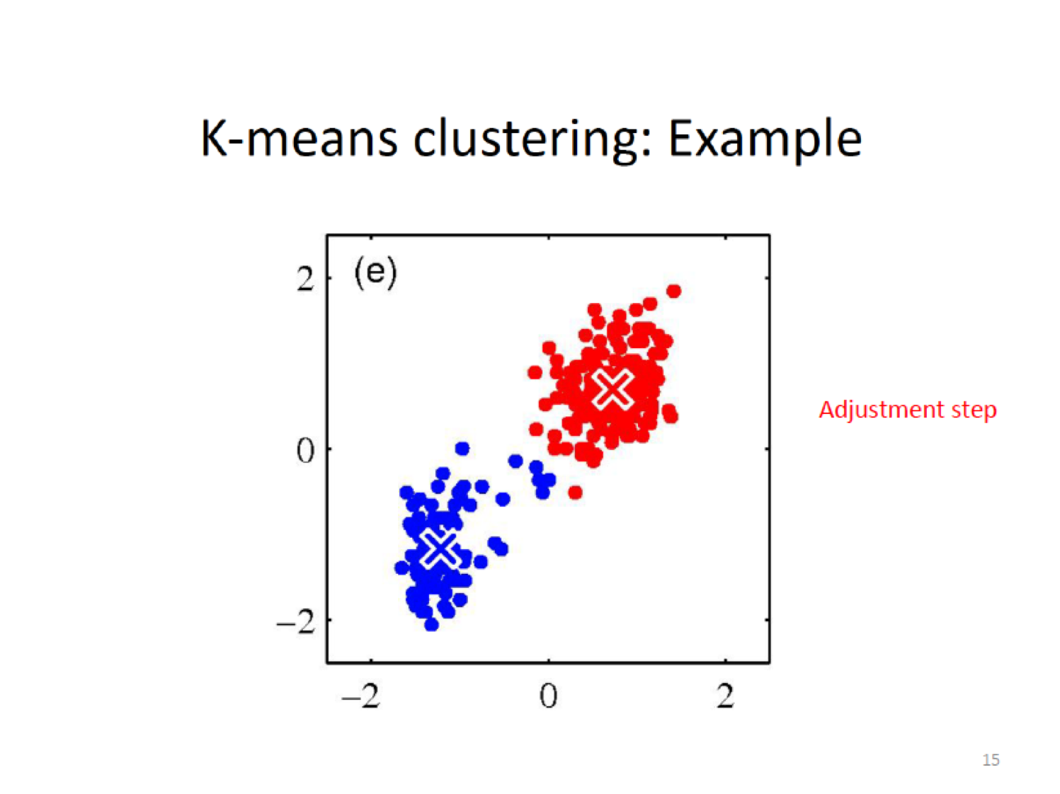
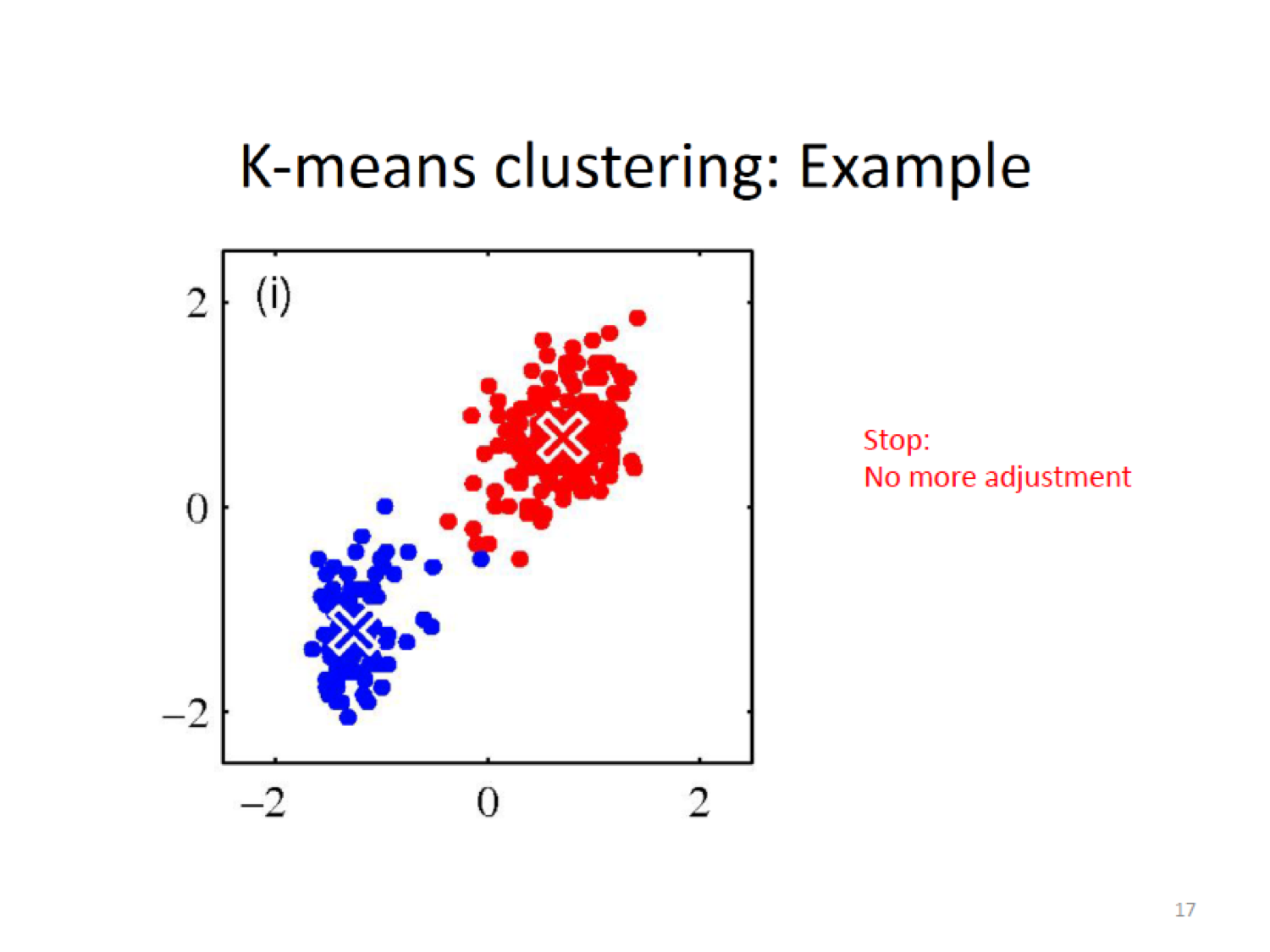
- Iterate the Assignment and Update steps until the assignments no longer change.
16.5.3 K-means Example
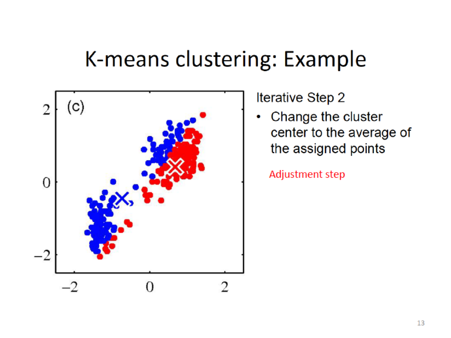 Here, we establish a new centroid (X) based on the means of the current assignment
Then do the assignment again by cacluting the closeness to the new centroid,
Here, we establish a new centroid (X) based on the means of the current assignment
Then do the assignment again by cacluting the closeness to the new centroid,
16.5.3.1 Snapshot of Algorithm
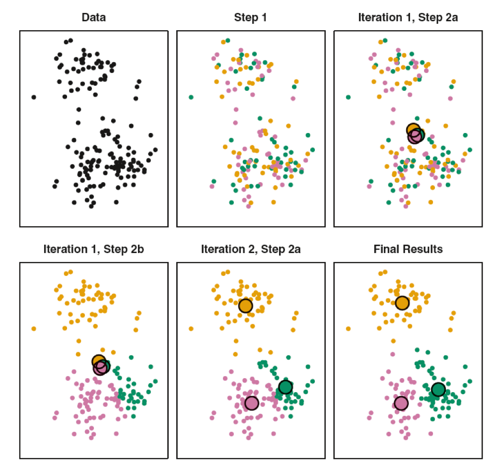 Randomness of the initial choice for the starting point. We might end up with different solutions when we have different starting points.
Now, let’s take a look with various random starting points.
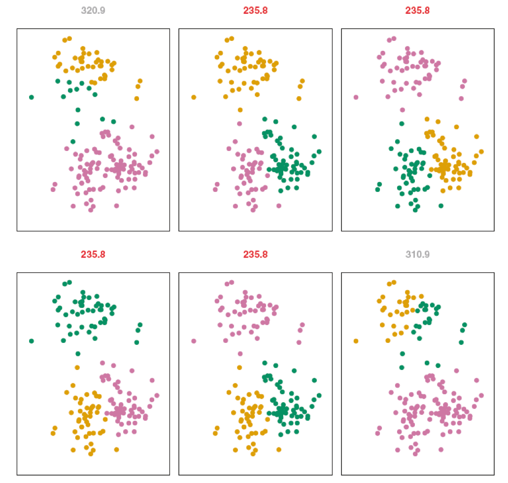
We ended up with three clusters, but the random start value influenced, above the variance is printed, there are 4 identical solutions \(235.8\) but different order (label switching) In R we can set a seed value so that they replicate.
16.5.3.2 Local Optimum
The K-Means algorithm finds a local rather than a global optimum. This means results obtained will depend on the initial (random) cluster assignment of each observation
It is important to run the algorithm multiple times from different random starting values and then select the best solution. Here, by best, we mean the minimum within cluster variance.
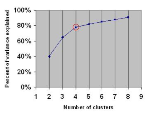
16.5.4 Choosing K
16.5.4.1 How to Choose \(K\)?
You want to maximize data reduction while making sure that you have good accuracy in terms of cluster memberships.
Some possibilities for choosing \(K\):
- Elbow method (see also within and between sum of squares in the R script)
- Information criterion approach (AIC, BIC, DIC)
- Two-step approach – using the dendogram from hierarchical clustering
- Using the Silhouette coefficient (see next)
16.5.4.2 Silhouette Coefficient
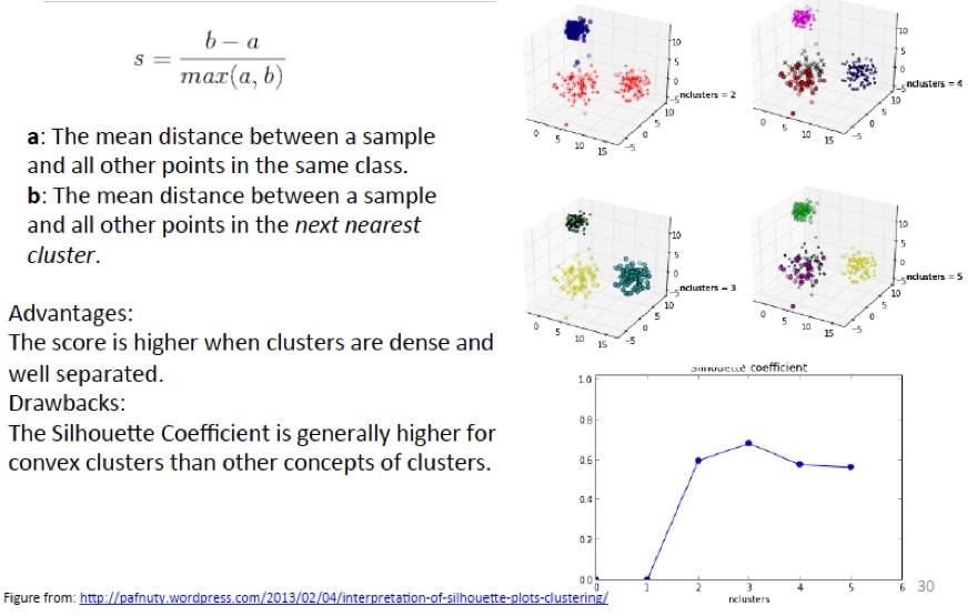 The silhouette coefficient is one such measure. It works as follows:
For each point \(p\), first find the average distance between p and all other points in the same cluster (this is a measure of cohesion, call it \(a\)). Then find the average distance between \(p\) and all points in the nearest cluster (this is a measure of separation from the closest other cluster, call it \(b\)). The silhouette coefficient for \(p\) is defined as the difference between \(b\) and \(a\) divided by the greater of the two (\(max(a,b)\)).
We evaluate the cluster coefficient of each point and from this we can obtain the ‘overall’ average cluster coefficient.
Intuitively, we are trying to measure the space between clusters. If cluster cohesion is good (\(a\) is small) and cluster separation is good (\(b\) is large), the numerator will be large, etc.
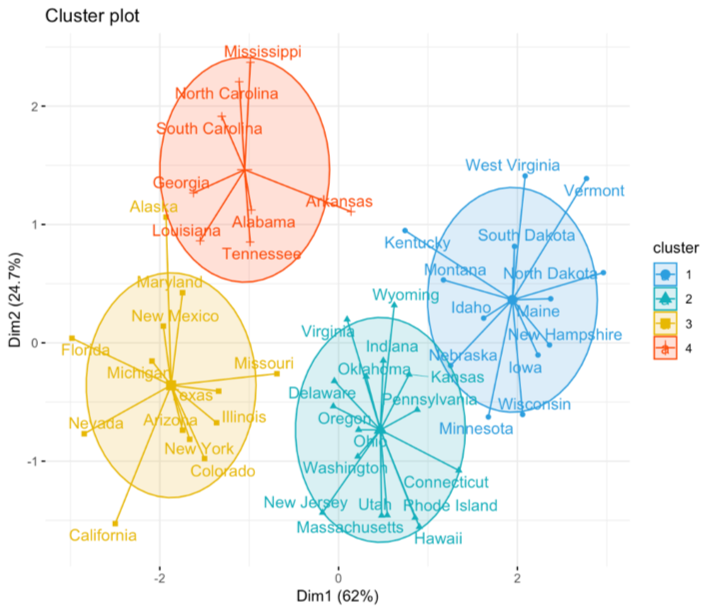
The silhouette plot shows the that the silhouette coefficient was highest when \(k = 3\), suggesting that’s the optimal number of clusters. In this example we are lucky to be able to visualize the data and we might agree that indeed, three clusters best captures the segmentation of this data set.
If we were unable to visualize the data, perhaps because of higher dimensionality, a silhouette plot would still give us a suggestion.