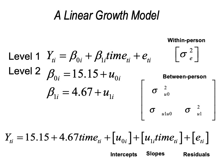
13.5 Linear Growth Model
Now let’s add in grade as a (time-varying) predictor. We look at the linear relation between the time variable (grade) and the outcome variable (verb).
13.5.1 Random Intercept Model
My naming convention for objects here is: fixed linear (fl) and random intercept (ri)
fl_ri_fit <- lme(
  fixed = verb ~ 1 + grade,
  random = ~ 1|id,
  data=verblong,
  na.action = na.exclude,
  method = "ML"
)
summary(fl_ri_fit)
## Linear mixed-effects model fit by maximum likelihood
## Data: verblong
## AIC BIC logLik
## 5225.662 5244.48 -2608.831
##
## Random effects:
## Formula: ~1 | id
## (Intercept) Residual
## StdDev: 6.295478 4.510587
##
## Fixed effects: verb ~ 1 + grade
## Value Std.Error DF t-value p-value
## (Intercept) 15.15099 0.5397641 611 28.06966 0
## grade 4.67339 0.0823294 611 56.76454 0
## Correlation:
## (Intr)
## grade -0.496
##
## Standardized Within-Group Residuals:
## Min Q1 Med Q3 Max
## -2.70731017 -0.54837346 -0.03479899 0.52061645 4.13309807
##
## Number of Observations: 816
## Number of Groups: 204Let’s look at the predicted trajectories from this model
#Place individual predictions and residuals into the dataframe
verblong$pred_fl_ri <- predict(fl_ri_fit)
verblong$resid_fl_ri <- residuals(fl_ri_fit)
#Create a function for the mean trajectory
fun_fl_ri <- function(x) { 15.15099 + 4.67339*x }

#plotting PREDICTED intraindividual change
ggplot(data = verblong, aes(x = grade, y = pred_fl_ri, group = id)) +
  ggtitle("Fixed Linear, Random Intercept") +
  #  geom_point() +
  geom_line() +
  xlab("Grade") +
  ylab("PREDICTED WISC Verbal Score") + ylim(0,100) +
  scale_x_continuous(breaks=seq(1,6,by=1)) +
  stat_function(fun=fun_fl_ri, color="red", size = 2) +
  theme_classic()
## Warning: Multiple drawing groups in `geom_function()`
## ℹ Did you use the correct group, colour, or fill aesthetics?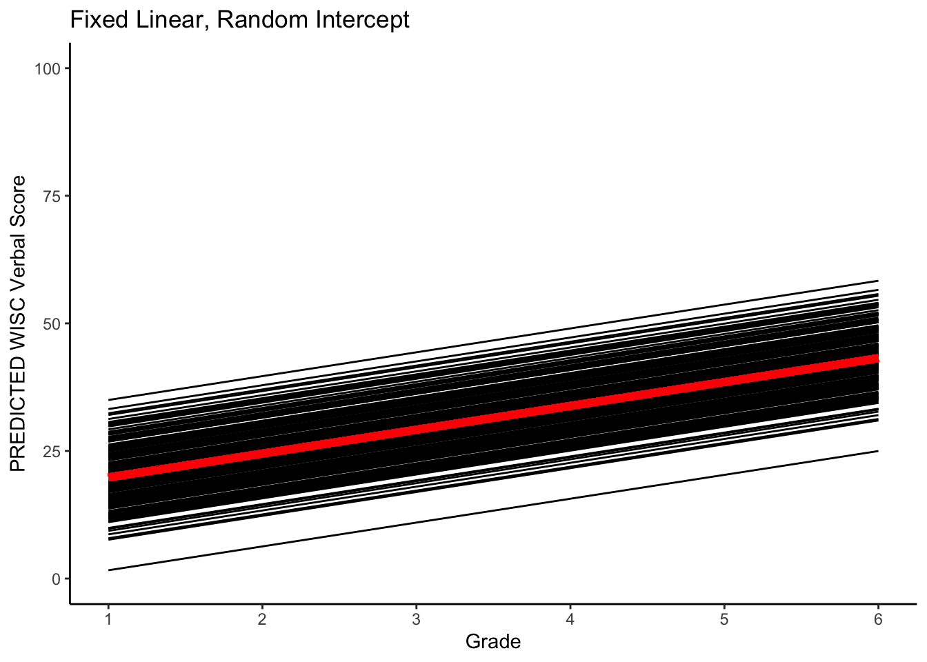
Note how all the lines are parallel. This imples individual variability in starting point but a constant rate of change over time.
Let’s look at the residuals.
ggplot(data = verblong, aes(x = grade, y = resid_fl_ri, group = id)) +
  ggtitle("Fixed Linear, Random Intercept") +
  #  geom_point() +
  geom_line() +
  xlab("Grade") +
  ylab("RESIDUAL WISC Verbal Score") +
  scale_x_continuous(breaks=seq(1,6,by=1)) +
  theme_classic()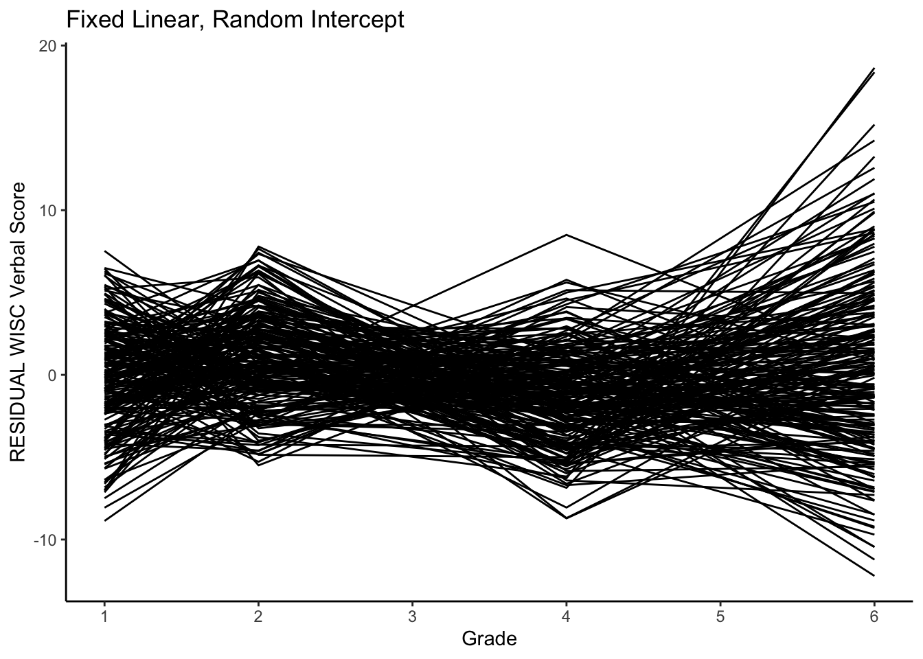
Note the differences in variance.
13.5.2 Random Intercept and Slopes Model
fl_rl_fit <- lme(
  fixed = verb ~ 1 + grade,
  random = ~ 1 + grade|id,
  data=verblong,
  na.action = na.exclude,
  method = "ML"
)
summary(fl_rl_fit)
## Linear mixed-effects model fit by maximum likelihood
## Data: verblong
## AIC BIC logLik
## 5050.844 5079.071 -2519.422
##
## Random effects:
## Formula: ~1 + grade | id
## Structure: General positive-definite, Log-Cholesky parametrization
## StdDev Corr
## (Intercept) 3.898138 (Intr)
## grade 1.236530 0.324
## Residual 3.581590
##
## Fixed effects: verb ~ 1 + grade
## Value Std.Error DF t-value p-value
## (Intercept) 15.15099 0.3681978 611 41.14905 0
## grade 4.67339 0.1085687 611 43.04546 0
## Correlation:
## (Intr)
## grade -0.155
##
## Standardized Within-Group Residuals:
## Min Q1 Med Q3 Max
## -2.61515107 -0.54356125 -0.02857262 0.52294871 3.17283564
##
## Number of Observations: 816
## Number of Groups: 204We can take a look at the ICCs to see if we are doing any better explaining the within-person variance.
RandomEffects <- as.numeric(VarCorr(fl_rl_fit)[,1])
ICC_between <- sum(RandomEffects[1:2])/sum(RandomEffects)
ICC_between
## [1] 0.5659288Let’s look at the predicted trajectories from this model. We can start by saving the predicted trajectories and residuals into our dataframe.
Next, we make a small function to plot the mean trajectory. Now we use the fixedf() function directly rather than type the numbers manually from the output.
#Create a function for the prototype
#fun_fl_rl <- function(x) {
#  15.15099 + 4.67339*x
#}

fun_fl_rl <- function(x) {
  fixef(fl_rl_fit)[[1]] + fixef(fl_rl_fit)[[2]]*x
}

#plotting PREDICTED intraindividual change
ggplot(data = verblong, aes(x = grade, y = pred_fl_rl, group = id)) +
  ggtitle("Fixed Linear, Random Linear") +
  #  geom_point() +
  geom_line() +
  xlab("Grade") +
  ylab("PREDICTED WISC Verbal Score") + ylim(0,100) +
  scale_x_continuous(breaks=seq(1,6,by=1)) +
  stat_function(fun=fun_fl_rl, color="red", size = 2) +
  theme_classic()
## Warning: Multiple drawing groups in `geom_function()`
## ℹ Did you use the correct group, colour, or fill aesthetics?
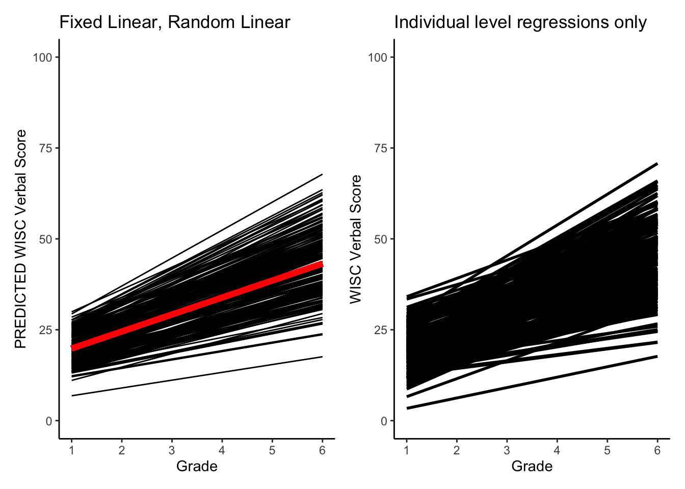
Note how the lines are no longer parallel. We now have a model that implies individual variability in the starting point and rate of change.
We can also plot the residuals.
#plotting RESIDUAL intraindividual change
ggplot(data = verblong, aes(x = grade, y = resid_fl_rl, group = id)) +
  ggtitle("Fixed Linear, Random Linear") +
  #  geom_point() +
  geom_line() +
  xlab("Grade") +
  ylab("RESIDUAL WISC Verbal Score") +
  scale_x_continuous(breaks=seq(1,6,by=1)) +
  theme_classic()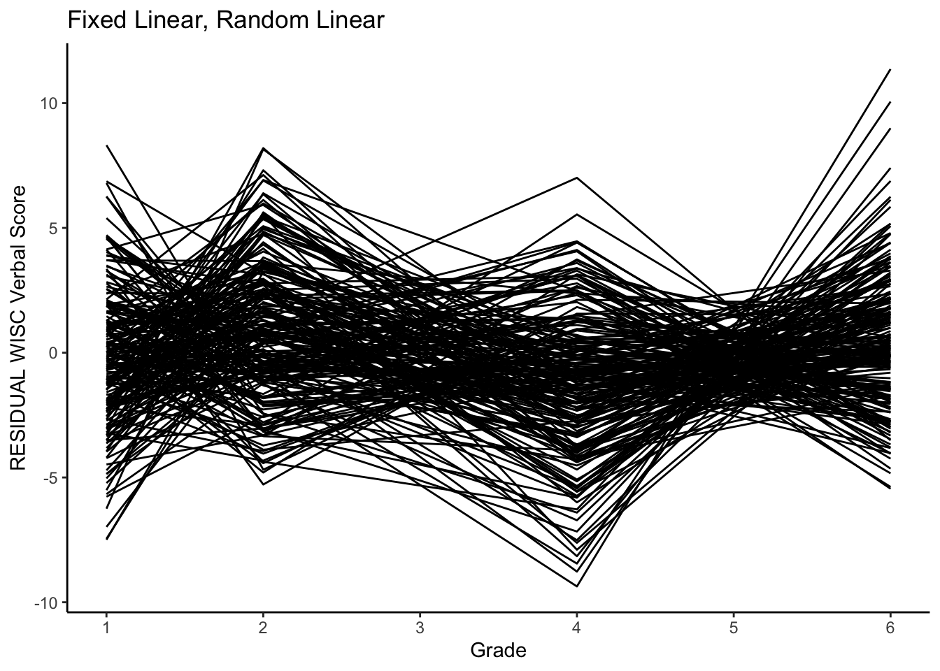
This model did a bit better on getting the residual variances similar at all grades (in line with assumptions).
13.5.3 Model Comparison
Let’s test the significance of having random slopes. We compare models by applying anova() function to examine difference in fit between the two nested models.
##           Model df      AIC      BIC    logLik   Test  L.Ratio p-value
## fl_ri_fit     1  4 5225.662 5244.480 -2608.831
## fl_rl_fit     2  6 5050.844 5079.071 -2519.422 1 vs 2 178.8176  <.0001
From the test results we see they are different. This provides a significance test for the variance and covariance (2 degrees of freedom).
13.5.4 MLM and Individual Models
Remember, earlier, we ran individual-level regressions.
##    id reg_1.(Intercept) reg_1.grade
## 1   1         15.940169    6.376102
## 2   2          5.232712    5.047627
## 3   3         26.838136    3.312881
## 4   4         19.493729    4.614237
## 5   5         19.145424    7.805254
## 6   6         11.554576    5.224746
## 7   7          2.903559    6.378136
## 8   8         14.198814    1.957288
## 9   9         10.816441    6.041864
## 10 10         18.385763    5.097458
## 11 11         16.319661    6.437797
## 12 12         12.089661    3.667797
Let’s also obtain individual-level estimates from the MLM model.
## (Intercept)       grade
## 15.15099 4.67339## (Intercept) grade
## 1 2.112943 1.23363573
## 2 -5.539718 -0.61673154
## 3 5.640183 0.09800779
## 4 2.526637 0.34162940
## 5 5.399309 2.49279594
## 6 -1.607547 0.06056857We add the fixed effect and random effect parameters together to get analogues of the individual-level parameters.
#Individual intercepts (MLM model based)
MLM_intercept <- FE[1] + RE[,1]
#Individual slopes (MLM model based)
MLM_grade <- FE[2] + RE[,2]
Let’s combine the individual regression intercepts and slopes and the model based intercepts and slopes together in order to compare.
indiv_parm_combined <- cbind(MLM_intercept,MLM_grade,indiv_reg_data[,2:3])
head(indiv_parm_combined)
## MLM_intercept MLM_grade reg_1.(Intercept) reg_1.grade
## 1 17.263936 5.907026 15.940169 6.376102
## 2 9.611275 4.056658 5.232712 5.047627
## 3 20.791176 4.771398 26.838136 3.312881
## 4 17.677629 5.015019 19.493729 4.614237
## 5 20.550302 7.166186 19.145424 7.805254
## 6 13.543446 4.733958 11.554576 5.224746Look at the descriptives statistics.
##                   vars   n  mean   sd median trimmed  mad  min   max range
## MLM_intercept        1 204 15.15 3.26  15.35   15.12 3.25 4.69 23.78 19.09
## MLM_grade            2 204  4.67 1.09   4.56    4.64 1.09 2.15  7.69  5.54
## reg_1.(Intercept)    3 204 15.15 5.27  15.14   15.23 5.12 0.50 29.41 28.91
## reg_1.grade          4 204  4.67 1.55   4.60    4.61 1.53 1.41  9.38  7.97
##                    skew kurtosis   se
## MLM_intercept      0.00    -0.23 0.23
## MLM_grade          0.26    -0.31 0.08
## reg_1.(Intercept) -0.08     0.06 0.37
## reg_1.grade 0.38 0.02 0.11## MLM_intercept MLM_grade reg_1.(Intercept) reg_1.grade
## MLM_intercept 1.00 0.68 0.89 0.31
## MLM_grade 0.68 1.00 0.27 0.91
## reg_1.(Intercept) 0.89 0.27 1.00 -0.16
## reg_1.grade 0.31 0.91 -0.16 1.00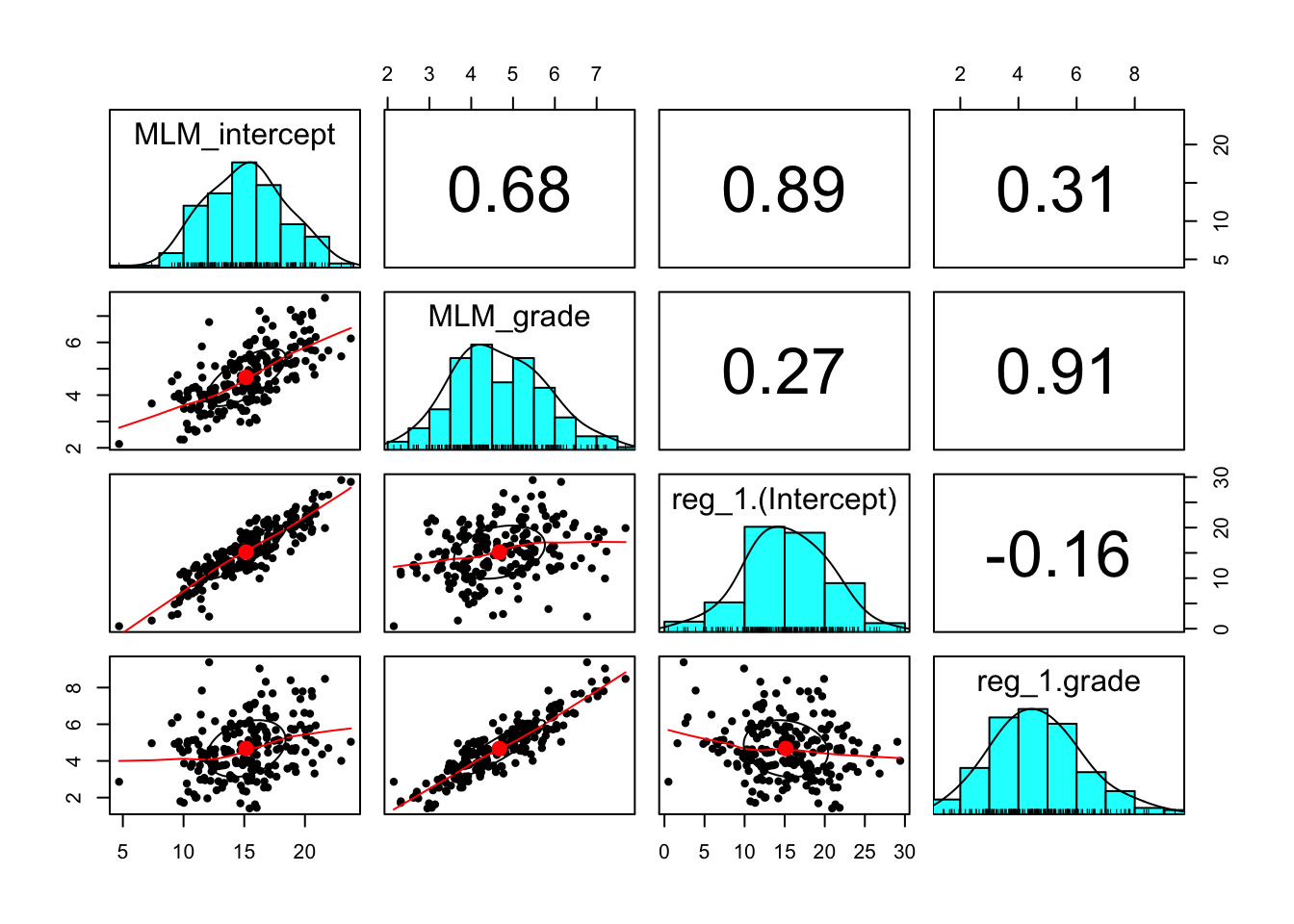
Let’s compare the two predictions. What do you notice?
library(see)
#plotting PREDICTED intraindividual change
GCMpred = ggplot(data = verblong, aes(x = grade, y = pred_fl_rl, group = id)) +
  ggtitle("Fixed Linear, Random Linear") +
  #  geom_point() +
  geom_line() +
  xlab("Grade") +
  ylab("PREDICTED WISC Verbal Score") + ylim(0,100) +
  scale_x_continuous(breaks=seq(1,6,by=1)) +
  stat_function(fun=fun_fl_rl, color="red", size = 2) +
  theme_classic()

#making intraindividual change plot
IndPred = ggplot(data = verblong, aes(x = grade, y = verb, group = id)) +
   ggtitle("Individual level regressions only") +
  geom_smooth(method=lm,se=FALSE,colour="black", size=1) +
  xlab("Grade") +
  ylab("WISC Verbal Score") + ylim(0,100) +
  scale_x_continuous(breaks=seq(1,6,by=1)) +
  theme_classic()

plots(GCMpred, IndPred)
## Warning: Multiple drawing groups in `geom_function()`
## ℹ Did you use the correct group, colour, or fill aesthetics?## `geom_smooth()` using formula = 'y ~ x'