17.3 The N=1 VAR Model
Consider extending our AR(1) model to include hours measurements of concentration (\(y_{1}\)) and fatigue (\(y_{1}\)). We now have a VAR(1) model where we are interested in two constructs, and their relation to eachother, across time.
Our interpretation of the AR parameter remains the same except now we also have cross-regressive parameters to consider (e.g. \(\alpha_{12}\) and \(\alpha_{21}\)).
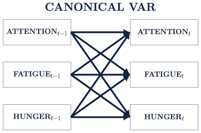
Interpretation of Directed Paths
- Auto-regressive paths (e.g. \(Attention_{t-1}\) -> \(Attention_{t}\) or \(\alpha_{11}\))
- AR parameters can be interpreted as a measure of inertia, stability or regulatory weakness.
- Cross-regressive paths (e.g. \(Attention_{t-1}\) -> \(Fatigue_{t}\)or \(\alpha_{21}\))
- cross-regressive paths indicate cross-construct influence, or buffering
The Vector Autoregressive (VAR) Model
In Economics widespread adoption of VAR models in the mid-1980s marked the beginning of a sea change in modeling and forecasting practice (Allen et al., 2006).
Advantages of the Unrestricted VAR Model
- Offers a concise interpretation of inter-variable relations
- Visualized easily using path or network connection diagrams
- Allow for the inclusion of many potentially relevant variables
Finally, we can extend the VAR model to handle additional variables we might think are related to our process of interest.
17.3.1 Fitting an VAR(1) Model in R
Now, let’s use the concentrate and fatigue variables.
Many software routines won’t require us to lag our data before prior to the analysis because this is done within the program itself. However, the process to lag our data for a multiple variable VAR model follows directly from the AR code.
first           <- df[1:(nrow(df)-1), ]
second          <- df[2:(nrow(df)  ), ]
lagged_df       <- data.frame(first, second)
colnames(lagged_df) <- c(paste0(colnames(df), "lag"), colnames(df))
head(lagged_df)
## concentratelag fatiguelag concentrate fatigue
## 1 33 62 31 50
## 2 31 50 30 36
## 3 30 36 33 39
## 4 33 39 34 71
## 5 34 71 22 47
## 6 22 47 27 43Now, we can use the vars package to fit a VAR(1) model for this single individual.
## $concentrate
##                   Estimate Std. Error    t value     Pr(>|t|)
## concentrate.l1  0.02448290 0.09686611  0.2527499 8.009375e-01
## fatigue.l1     -0.01819429 0.08733041 -0.2083386 8.353534e-01
## const          38.00889080 4.87657767  7.7941732 4.109929e-12
##
## $fatigue
##                  Estimate Std. Error  t value     Pr(>|t|)
## concentrate.l1  0.1142125 0.09895499 1.154186 0.2509481959
## fatigue.l1      0.3522671 0.08921366 3.948579 0.0001396888
## const          19.2844903 4.98173908 3.871036 0.0001850659
transition_mat <- as.matrix(do.call("rbind",lapply(seq_along(colnames(df)), function(x) {
fit$varresult[[x]]$coefficients
})))
rownames(transition_mat) <- colnames(df)
transition_mat## concentrate.l1 fatigue.l1 const
## concentrate 0.0244829 -0.01819429 38.00889
## fatigue 0.1142125 0.35226713 19.2844917.3.2 Stationarity and Non-Stationarity
Consider a multivariate time series, \(\{\mathbf{X}_{t}\}_{t \in \mathbb{Z}} = \{(X_{j,t})_{j=1,\dots,d}\}\), that follows a vector autoregressive model of order \(p\), \[ \label{varp1} \mathbf{X}_{t} = \boldsymbol{\Phi}_{1} \mathbf{X}_{t-1} + \ldots + \boldsymbol{\Phi}_{p} \mathbf{X}_{t-p} + \boldsymbol{\varepsilon}_{t}, \quad t \in \mathbb{Z}. \]
- \(\boldsymbol{\Phi}_{1}, \dots, \boldsymbol{\Phi}_{p}\) are \(d \times d\) transition matrices.
- \(\boldsymbol{\varepsilon}_{t}\) is a white noise series, \(\{\boldsymbol{\varepsilon}_{t}\}_{t \in \mathbb{Z}} \sim \text{WN}(\mathbf{0}, \boldsymbol{\Sigma}_{\boldsymbol{\varepsilon}})\) with \(\mathbb{E}(\boldsymbol{\varepsilon}_{t})=0\), \(\mathbb{E}(\boldsymbol{\varepsilon}_{t}\boldsymbol{\varepsilon}_{s}^{'})=0\) for \(s \neq t\).
- For simplicity we assume \(\mathbf{X}_{t}\) is of zero mean and \(\eqref{varp1}\) satisfies the stability conditions discussed earlier.
As we showed earlier it is common to estimate \(\eqref{varp1}\) using ordinary least-squares (OLS) regression, \[ (\widehat{\boldsymbol{\Phi}}_1,\ldots,\widehat{\boldsymbol{\Phi}}_p) = \argmin_{\boldsymbol{\Phi}_1,\ldots,\boldsymbol{\Phi}_p} \sum_{t=p+1}^T \| \mathbf{X}_t - \boldsymbol{\Phi}_1 \mathbf{X}_{t-1} - \ldots - \boldsymbol{\Phi}_p \mathbf{X}_{t-p}\|_{2}^2. \] where a unique stationary solution can be found when the eigenvalues of \(\boldsymbol{\Phi}\) are smaller than one in absolute value.
non_stationary_AR <- matrix(c(1,2,3,4), 2, 2)
stationary_AR <- matrix(c(.1,.2,.3,.4), 2, 2)
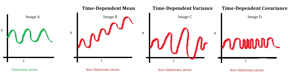
max(abs(eigen(non_stationary_AR)$values)) < 1## [1] FALSE## [1] TRUEPerhaps more importantly, what do stationary and non-stationary series look like? Here are some simplistic examples
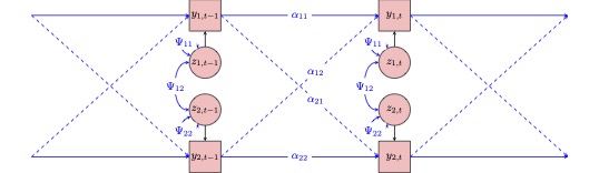
17.3.3 A Note on path Diagrams
Both examples below represent bivariate VAR(1) models. It is important to be comfortable with both representations as they are each commonly presented in the literature. Note the two diagrams primarily difer in how they represent the autorgressive and cross-regressive effects. In Path Diagram 1, both are illustrated using directed arrows. In Path Diagram 2, autoregressive paths are indicated by directed self-loops, while cross-regressive paths are indicated by directed arrows.
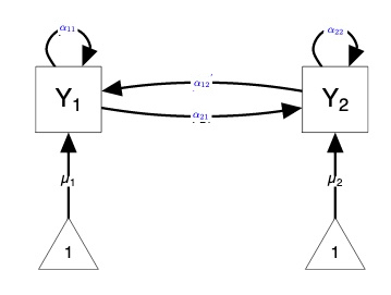
Note that Path Diagram 1 does not include information about the means (intercepts), which is indicated by the triangles in Path Diagram 2. Likewise, Path Diagram 2 does not include a visual depiction of the errors, indicated by \(z_{1}\) and \(z_{2}\) in Path Diagram 1.