9.5 Single Predictor Model
9.5.2 Single Predictor Model in GLM
Let’s fit a single predictor Poisson regression model for morbidity at Wave 1 using income bracket as our predictor. For now let’s treat income bracket as a continuous predictor.
Note for the Poisson regression we use family = poisson(link=log) argument.
model1 <- glm(
  formula = morbidityw1 ~ 1 + income_star,
  family = poisson(link=log),
  data = ferraro2016,
  na.action = na.exclude
)##
## Call:
## glm(formula = morbidityw1 ~ 1 + income_star, family = poisson(link = log),
## data = ferraro2016, na.action = na.exclude)
##
## Coefficients:
## Estimate Std. Error z value Pr(>|z|)
## (Intercept) 1.007472 0.011047 91.195 < 2e-16 ***
## income_star -0.032445 0.007838 -4.139 3.48e-05 ***
## ---
## Signif. codes: 0 '***' 0.001 '**' 0.01 '*' 0.05 '.' 0.1 ' ' 1
##
## (Dispersion parameter for poisson family taken to be 1)
##
## Null deviance: 8166.6 on 2994 degrees of freedom
## Residual deviance: 8149.5 on 2993 degrees of freedom
## (27 observations deleted due to missingness)
## AIC: 14986
##
## Number of Fisher Scoring iterations: 59.5.3 Deviance and Goodness of Fit
##
## Call:
## glm(formula = morbidityw1 ~ 1 + income_star, family = poisson(link = log),
##     data = ferraro2016, na.action = na.exclude)
##
## Coefficients:
##              Estimate Std. Error z value Pr(>|z|)
## (Intercept)  1.007472   0.011047  91.195  < 2e-16 ***
## income_star -0.032445   0.007838  -4.139 3.48e-05 ***
## ---
## Signif. codes:  0 '***' 0.001 '**' 0.01 '*' 0.05 '.' 0.1 ' ' 1
##
## (Dispersion parameter for poisson family taken to be 1)
##
##     Null deviance: 8166.6  on 2994  degrees of freedom
## Residual deviance: 8149.5  on 2993  degrees of freedom
##   (27 observations deleted due to missingness)
## AIC: 14986
##
## Number of Fisher Scoring iterations: 5We can think about the deviance as a measure of how well the model fits the data.
- If the model fits well, the observed values \(Y_{i}\) will be close to their predicted means \(\mu_{i}\), causing the deviance to be small.
- If this value greatly exceeds one, it may be indicative of overdispersion.
The rationale for this heuristic is based on the fact that the residual deviance is \(\chi^2_k\) distributed with mean equal to the degrees of freedom (n-p). Instead of using this rule of thumb it is just as simple to formulate a goodness-of-fit test for our model as follows
## [1] 0The test of the model’s deviance is a test of the model against the null model. The null hypothesis is the fitted model fits the data as well as the saturated model. In this case, rejecting the null hypothesis (e.g. \(p > 0.05\)), indicates the Poisson model does not fit well. For more information see this wonderful post on stackexchange: https://stats.stackexchange.com/a/531484.
9.5.4 Overdispersion?
The deviance statistic suggests there may be a problem with overdispersion?
Overdispersion indicates there is greater variability in the data than would be expected based on the model.
Overdispersion is often encountered when fitting simple Poisson regression models. The Poisson distribution has one free parameter and does not allow for the variance to be adjusted independently of the mean.
If overdispersion is present the resultant model may yield biased parameter estimates and underestimated standard errors, possibly leading to invalid conclusions.
9.5.5 Interpretation of Single Predictor Model
How do we interpret the coefficients from our single predictor poisson regression?
In the classic linear regression model we might interpret a slope coefficient as characterizing the change in mean number of health problems for a 1-unit increase in income.
In our Poisson regression we are modeling the log of the mean number of health problems, so we must convert back to original units.
Intercept in Log Units
This is the Poisson regression estimate when all variables in the model are evaluated at zero. For our model, we have centered the income variable. This means for an individual with an average income level the log of the expected count for health problems is \(1.007\) units.
Intercept in Count Units
We can also exponentiate the intercept, \(exp(1.007) = 2.7\) indicating that at Wave 1 follow-up, an individual with an average income level is expected to have approximately \(2.7\) health problems.
9.5.5.1 Slope Coefficient
Slope Coefficient in Log Units
Within our single predictor model, \(b_1\) is the difference in log number of health problems for a 1-level difference in income bracket.
For example, consider a comparison of two models—one for a given income bracket \((x)\), and one income bracket higher \((x+1)\):
\[\begin{equation} \begin{split} log(\mu_X) &= \beta_0 + \beta_1X \\ log(\mu_{X+1}) &= \beta_0 + \beta_1(X+1) \\ log(\mu_{X+1})-log(\mu_X) &= \beta_1 \\ log \left(\frac{\mu_{X+1}}{\mu_X}\right) &= \beta_1\\ \frac{\mu_{X+1}}{\mu_X} &= e^{\beta_1} \end{split} \tag{4.1} \end{equation}\]
These results suggest that by exponentiating the coefficient of income, we obtain the multiplicative factor by which the mean count of health problems change. In this case, the mean number of health problems changes by a factor of \(e^{(-0.032445)}=0.968\).
We might also think about percent change as in Section 9.3.3. Here we would \(1-e^{(-0.032445)}*100=3.19\) percent decrease in the number of health problems for a 1-unit increase in income band.
To calculate the percentage change you can use the formulas in Section 9.3.3 or use the catregs package on github.
# manual
#(1-exp(coef(model1)[2]))*100 # if slope is negative, % decrease
#(exp(coef(model1)[1])-1)*100 # if slope is positive, % increase

# using catregs
#devtools::install_github("dmmelamed/catregs")
catregs::list.coef(model1)
## variables b SE z ll ul p.val exp.b ll.exp.b ul.exp.b
## 1 (Intercept) 1.007 0.011 91.195 0.986 1.029 0 2.739 2.680 2.799
## 2 income_star -0.032 0.008 -4.139 -0.048 -0.017 0 0.968 0.953 0.983
## percent CI
## 1 173.867 95 %
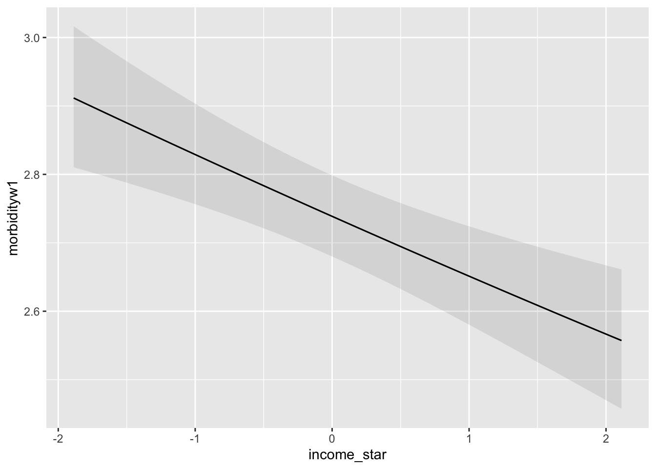
## 2 -3.192 95 %Marginal Effects
Let’s turn to the marginaleffects (Arel-Bundock 2022) package to look at the marginal effects of income on health.