13.4 Unconditional Means Model
We will begin by fitting the unconditional means model, or no growth model to the 4-ocasion WISC data.
We use the nlme package for fitting mixed effects models, also known as multilevel (MLM) or hierarchical linear models (HLM).
Specifically, we use the lme() function to fits the MLMs:
- The ‘fixed’ argument takes the fixed model
- The ‘random’ argument takes the random model
- The ‘data’ argument specifies the data sources
- The ‘na.action’ argument specifies how to handle missing data
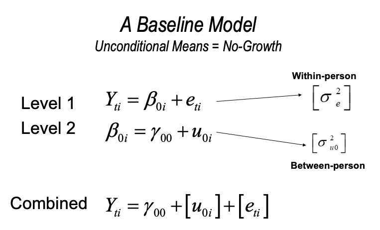
The Unconditional Means model contains a fixed and random intercept only. You can use the constant 1 to designate that only intercepts are being modeled.
um_fit <- lme(
  fixed= verb ~ 1,
  random = ~ 1|id,
  data = verblong,
  na.action = na.exclude,
  method = "ML"
)

summary(um_fit)
## Linear mixed-effects model fit by maximum likelihood
## Data: verblong
## AIC BIC logLik
## 6347.936 6362.05 -3170.968
##
## Random effects:
## Formula: ~1 | id
## (Intercept) Residual
## StdDev: 3.575939 11.30169
##
## Fixed effects: verb ~ 1
## Value Std.Error DF t-value p-value
## (Intercept) 30.33951 0.4684887 612 64.76039 0
##
## Standardized Within-Group Residuals:
## Min Q1 Med Q3 Max
## -1.9419919 -0.7619298 -0.1621987 0.5568904 3.3055064
##
## Number of Observations: 816
## Number of Groups: 204Let’s extract the random effects with the VarCorr() function
## id = pdLogChol(1)
##             Variance  StdDev
## (Intercept)  12.78734  3.575939
## Residual    127.72821 11.301691
We can compute the intra-class correlation (ICC) as the ratio of the random intercept variance (between-person) to the total variance (between + within), that includes the error.
First let’s store the variance estimates, which will be the first column of the VarCorr object (see above).
## [1] 12.78734 127.72821Next let’s compute the ICC. It is the ratio of the random intercept variance (between-person var) over the total variance (between + within var).
## [1] 0.09100302From the results we seeM there is lots of within-person variance for us to explain.
- between-person variance = \(9.2\%\)
- within-person variance = \(100 - 9.2 = 91.8\%\)
13.4.1 Predicted Trajectories
Place individual predictions and residuals from the unconditional means model um_fit into the dataframe
##     id grade  verb grad momed  pred_um   resid_um
## 1.1  1     1 24.42    0   9.5 32.14754  -7.727545
## 1.2  1     2 26.98    0   9.5 32.14754  -5.167545
## 1.4  1     4 39.61    0   9.5 32.14754   7.462455
## 1.6  1     6 55.64    0   9.5 32.14754  23.492455
## 2.1  2     1 12.44    0   5.5 27.85120 -15.411203
## 2.2  2     2 14.38    0   5.5 27.85120 -13.471203
We can make plots of the model outputs. Here we plot the between-person differences in levels (\(9\%\)).
ggplot(data = verblong, aes(x = grade, y = pred_um, group = id)) +
  ggtitle("Unconditional Means Model") +
#  geom_point() +
  geom_line() +
  xlab("Grade") +
  ylab("PREDICTED WISC Verbal Score") + ylim(0,100) +
  scale_x_continuous(breaks=seq(1,6,by=1)) +
  theme_classic()
Here we plot the between-person differences in levels (\(91\%\)).
#plotting RESIDUAL intraindividual change
ggplot(data = verblong, aes(x = grade, y = resid_um, group = id)) +
  ggtitle("Unconditional Means Model (residuals)") +
#  geom_point() +
  geom_line() +
  xlab("Grade") +
  ylab("RESIDUAL WISC Verbal Score") + #ylim(0,100) + Note the removal of limits on y-axis
  scale_x_continuous(breaks=seq(1,6,by=1)) +
  theme_classic()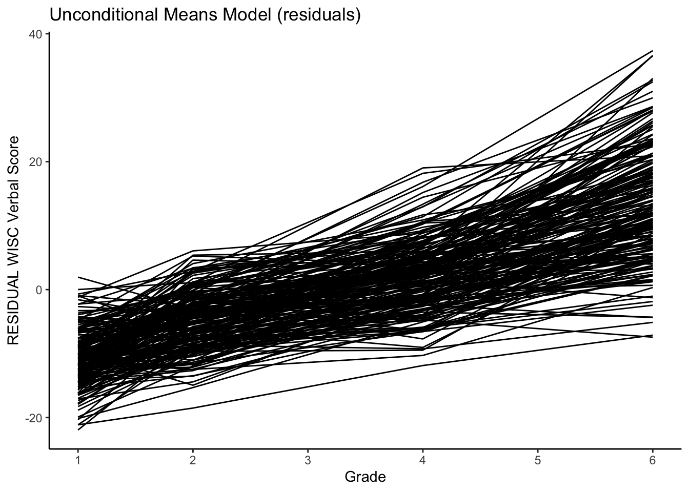
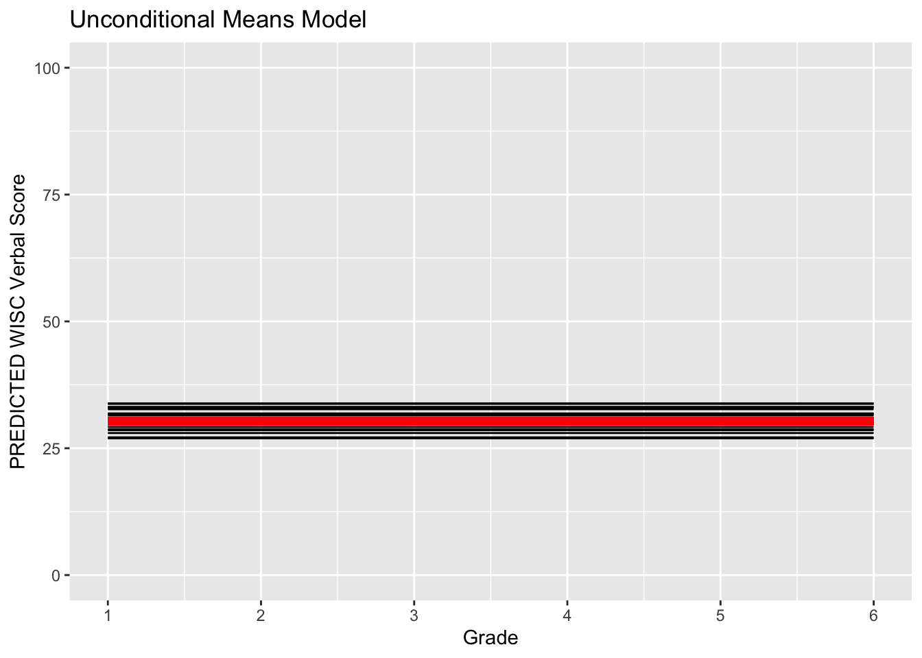
We cab also plot the predicted intraindividual change alongside the mean trajectory.
fun_um <- function(x) { 30.33951 + 0*x }
ggplot(data = verblong, aes(x = grade, y = pred_um, group = id)) +
  ggtitle("Unconditional Means Model") +
  #  geom_point() +
  geom_line() +
  xlab("Grade") +
  ylab("PREDICTED WISC Verbal Score") + ylim(0,100) +
  scale_x_continuous(breaks=seq(1,6,by=1)) +
  stat_function(fun=fun_um, color="red", size = 2) +
  theme_classic()
## Warning: Multiple drawing groups in `geom_function()`
## ℹ Did you use the correct group, colour, or fill aesthetics?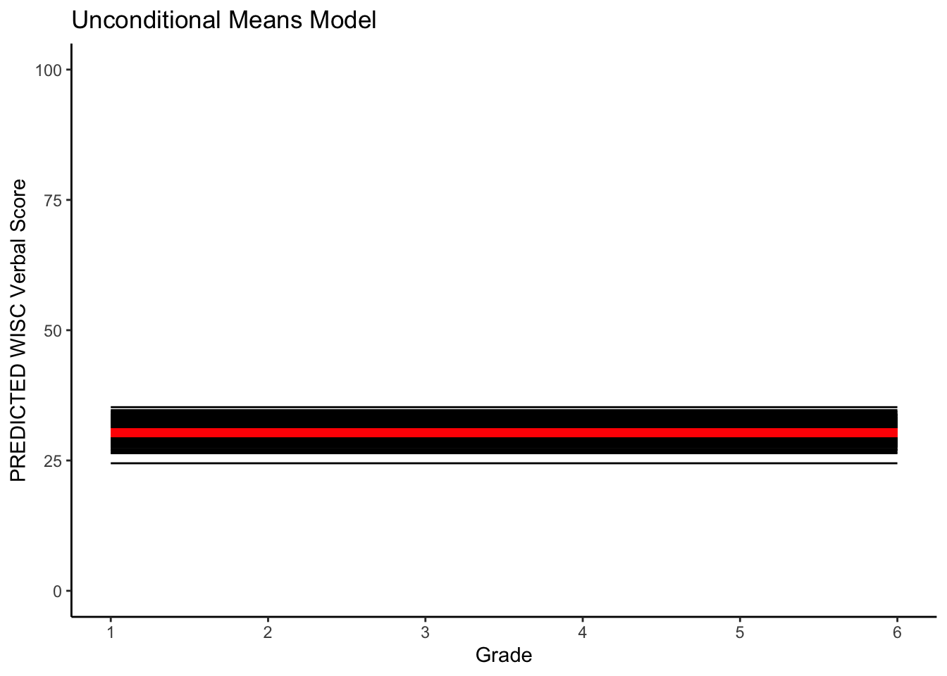
Since it is often too messy to plot all individuals we can also subset the plot.
randomsample <- sample(verblong$id,20)
ggplot(data = verblong[verblong$id %in% randomsample,], aes(x = grade, y = pred_um, group = id)) +
  ggtitle("Unconditional Means Model") +
  #  geom_point() +
  geom_line() +
  xlab("Grade") +
  ylab("PREDICTED WISC Verbal Score") + ylim(0,100) +
  scale_x_continuous(breaks=seq(1,6,by=1)) +
  stat_function(fun=fun_um, color="red", size = 2)
## Warning: Multiple drawing groups in `geom_function()`
## ℹ Did you use the correct group, colour, or fill aesthetics?