8.7 Marginal Effects
So far we have considered two possibilities for interpreting logistic regression results:
- Interpreting the log-odds directly
- Transforming the log-odds into odds
- A probability metric (for a single explanatory variable)
However, as we include more covariates in our model, interpretation becomes more difficult. We can only think about “holding other variable constant” in the log-odds and odds scale. For nonlinear model marginal effects provide us with an intuitive and easy to interpret method for understanding and communicating results.
8.7.1 A Definition of Marginal Effects
Marginal effects are partial derivatives of the regression equation with respect to each variable in the model for each unit in the data.
Put differently, the marginal effect measures the association between a change in an explanatory variable and a change in the response. The marginal effect is the slope of the prediction function, measured at a specific value of the explanatory variable.
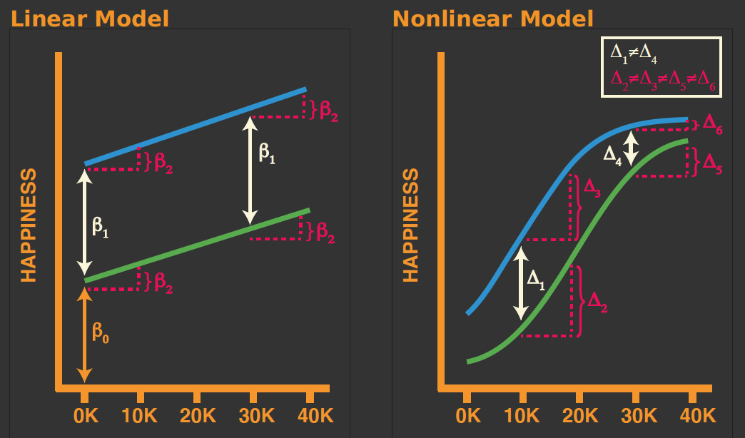
In linear models the effect of a given change in an independent variable is the same regardless of (1) the value of that variable at the start of its change, and (2) the level of the other variables in the model.
In nonlinear models the effect of a given change in an independent variable (1) depends on the values of other variables in the model, and (2) is no longer equal to the parameter itself.
Consider a linear and nonlinear model for happiness as a function of personal spending and a dummy variable indicating whether someone is rich.
8.7.2 A Few Observations
For the linear model: - Whether one is rich or poor does no impact the relationship between happiness and personal spending. - Differences in happiness levels between rich and poor are not dependent on the amount of money one spends.
From the nonlinear model: - Whether one is rich or poor does impact the relationship between happiness and personal spending. - Differences in happiness levels between rich and poor are dependent on the amount of money one spends.
8.7.2.1 Another Nonlinear Example
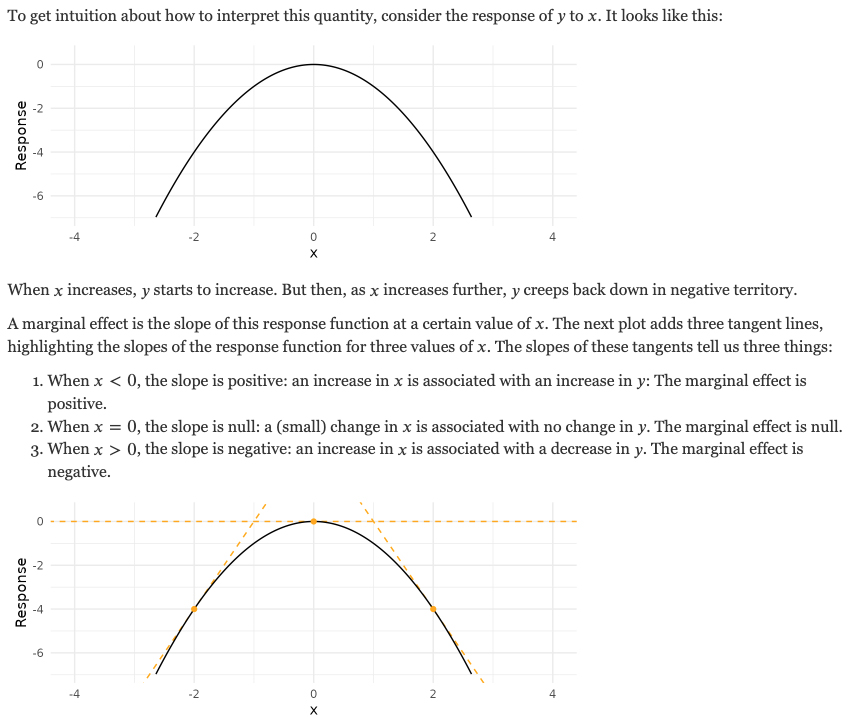
A helpful example is provided in the marginaleffects vignette.
Consider a simple quadratic
\[ y = -x^2 \\ \]
with partial derivative of \(y\) with respect to \(x\)
\[ \frac{\partial y}{\partial x} = -2x. \]
8.7.3 Types of Marginal Effects
There are generally three types of marginal effects people consider:
- Marginal Effects at the Means (MEM)
- Average Marginal Effects (AME)
- Marginal Effects at Representative Values (MEM)
We will focus on marginal effects at representative values as this is the most powerful option.
8.7.4 Example Model
Let’s fit a more complicated model. To look at marginal effects we will use the marginaleffects package.
## Warning: package 'marginaleffects' was built under R version 4.4.1model11 <- glm(Happy ~ 1 + PersonalSpending + ProsocialSpending + Income,
family = "binomial",
data = dunn2008,
na.action = na.exclude)
summary(model11)##
## Call:
## glm(formula = Happy ~ 1 + PersonalSpending + ProsocialSpending +
## Income, family = "binomial", data = dunn2008, na.action = na.exclude)
##
## Coefficients:
## Estimate Std. Error z value Pr(>|z|)
## (Intercept) -0.636366 0.223151 -2.852 0.00435 **
## PersonalSpending -0.011635 0.006643 -1.752 0.07985 .
## ProsocialSpending 0.083741 0.032975 2.540 0.01110 *
## Income20-35K -0.331327 0.288006 -1.150 0.24997
## Income35-50K -0.057632 0.297299 -0.194 0.84629
## Income50-65K 0.170117 0.326317 0.521 0.60214
## Income65-80K 0.221637 0.323873 0.684 0.49376
## Income> 80K 0.259641 0.307140 0.845 0.39791
## ---
## Signif. codes: 0 '***' 0.001 '**' 0.01 '*' 0.05 '.' 0.1 ' ' 1
##
## (Dispersion parameter for binomial family taken to be 1)
##
## Null deviance: 805.02 on 631 degrees of freedom
## Residual deviance: 791.06 on 624 degrees of freedom
## AIC: 807.06
##
## Number of Fisher Scoring iterations: 48.7.5 Marginal Effects at Representative Values (MER)
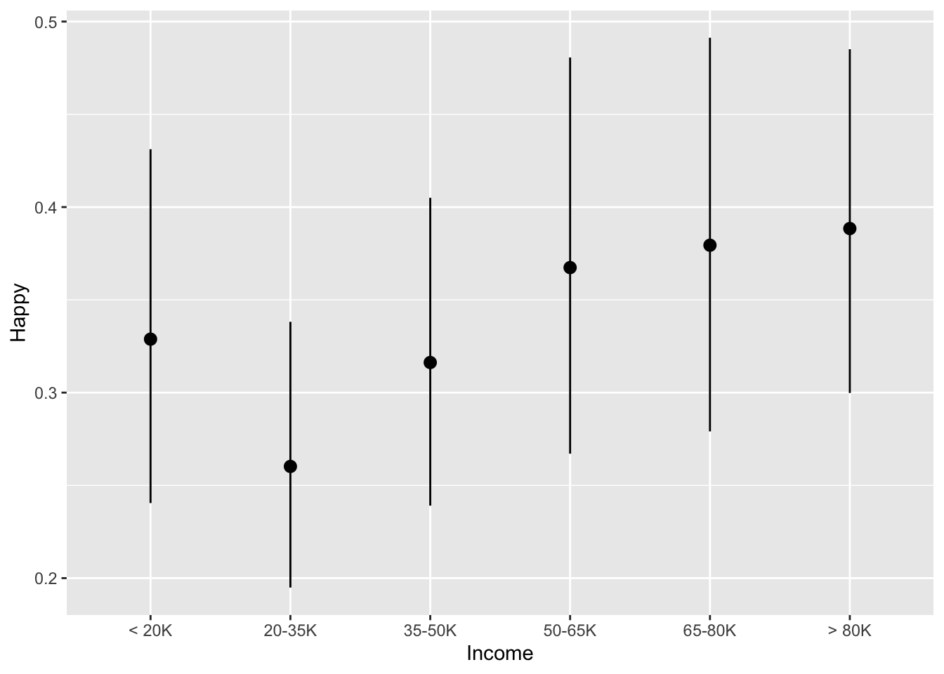
For example, let’s look at the impact of Income on the probability of being happy.
What if we were interested in the relationship between Income and PersonalSpending on the probability of being happy.
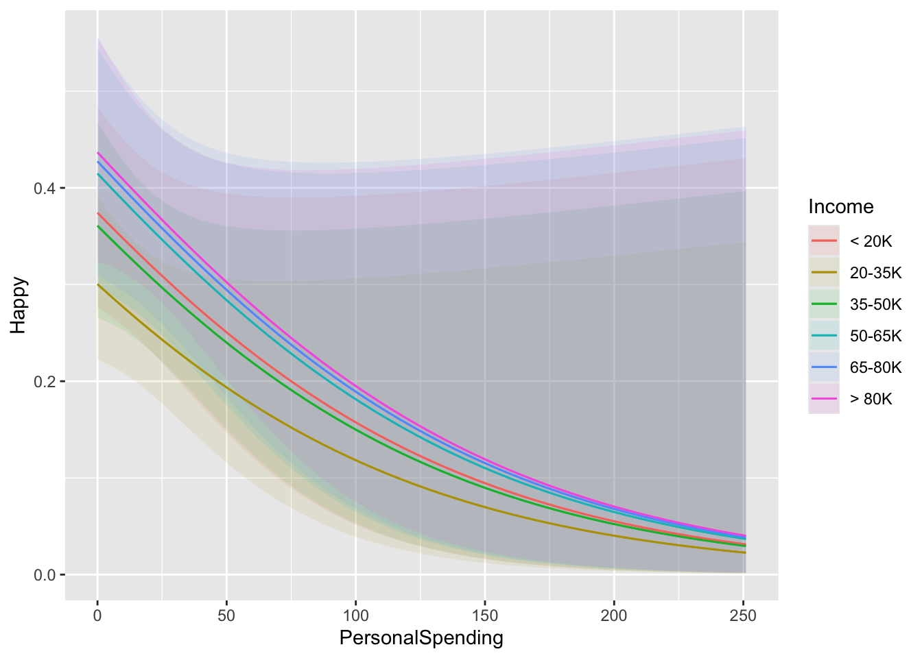
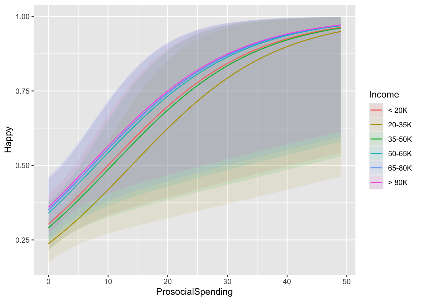
What if we were interested in the relationship between Income and ProsocialSpending on the probability of being happy.
In nonlinear, the marginal effect of one variable is conditional on the value of the other variable. This function draws a plot of the marginal effect of the effect variable for different values of the condition variable.
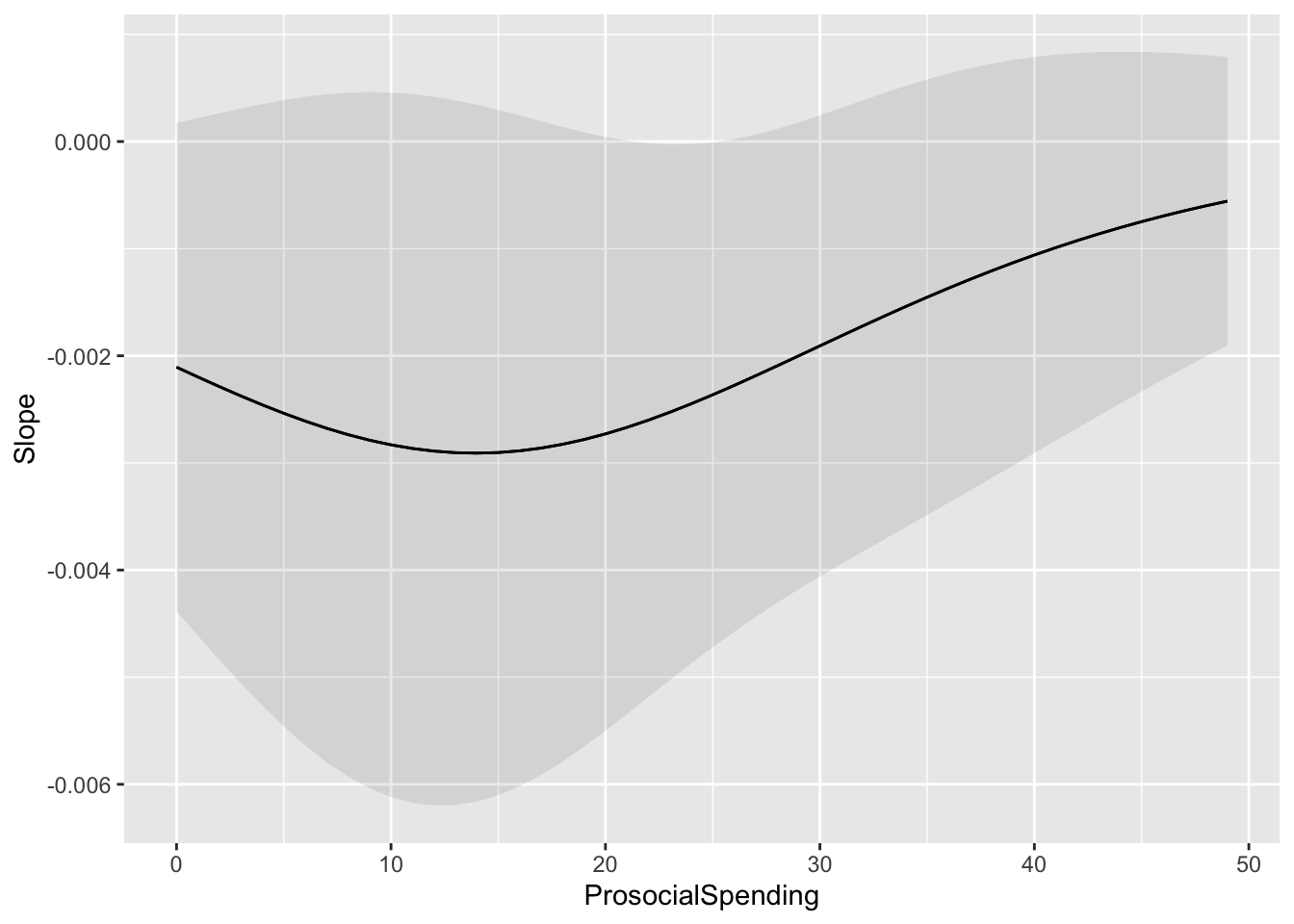
Let’s look at the effect of PersonalSpending on the relationship between ProsocialSpending and Happy.
marginaleffects::plot_slopes(model11, variables = "ProsocialSpending", condition = "PersonalSpending")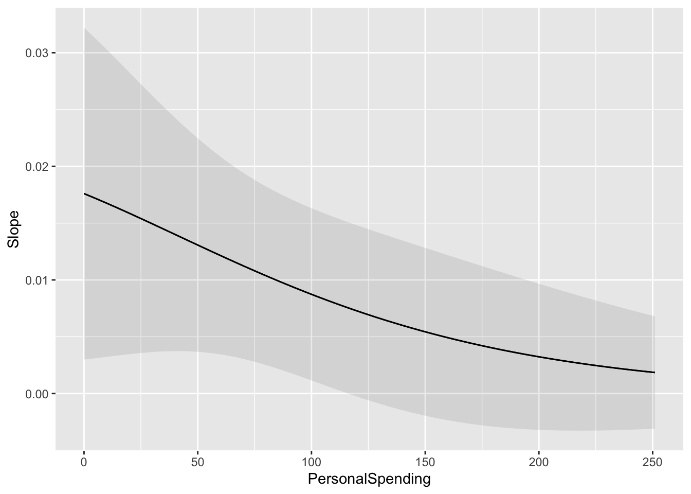
In addition, we can look at the effect of PersonalSpending on the relationship between PersonalSpending and Happy.
marginaleffects::plot_slopes(model11, variables = "PersonalSpending", condition = "ProsocialSpending")