12.2 Example Data

Loading some new libraries used in this chapter.

library(psych)     # for descriptives etc
library(ggplot2)   # for plotting
library(nlme)      # for mixed effects models
library(lme4)      # for mixed effects models
library(lmerTest)  # to get significance tests from lmer

12.2.1 Data Preparation and Description

For our examples, we use 3-occasion WISC data that are equally spaced.

Load the repeated measures data

filepath <- "https://quantdev.ssri.psu.edu/sites/qdev/files/wisc3raw.csv"
wisc3raw <- read.csv(file=url(filepath),header=TRUE)

Next, let’s Subset the variables of interest. For this chapter we will include:

• 3-occasion equally spaced repeated measures (verb2, verb4, verb6)
• A person-level grouping variable (grade)
• An ID variable (id)

After subsetting let’s take a look at some basic descriptives.

varnames <- c("id","verb2","verb4","verb6","grad")
wiscsub <- wisc3raw[ ,varnames]
describe(wiscsub)

##       vars   n   mean    sd median trimmed   mad   min    max  range  skew
## id       1 204 102.50 59.03 102.50  102.50 75.61  1.00 204.00 203.00  0.00
## verb2    2 204  25.42  6.11  25.98   25.40  6.57  5.95  39.85  33.90 -0.06
## verb4    3 204  32.61  7.32  32.82   32.42  7.18 12.60  52.84  40.24  0.23
## verb6    4 204  43.75 10.67  42.55   43.46 11.30 17.35  72.59  55.24  0.24
## grad     5 204   0.23  0.42   0.00    0.16  0.00  0.00   1.00   1.00  1.30
##       kurtosis   se
## id       -1.22 4.13
## verb2    -0.34 0.43
## verb4    -0.08 0.51
## verb6    -0.36 0.75
## grad     -0.30 0.03

Multilevel modeling analyses typically require a long data set. So, we also reshape from wide to long in order to have a long data set.

verblong <- reshape(
  data = wiscsub, 
  varying = c("verb2","verb4","verb6"), 
  timevar = "grade", 
  idvar = "id", 
  direction = "long", 
  sep = ""
)
verblong <- verblong[order(verblong$id,verblong$grade), c("id","grade","verb","grad")]
head(verblong,12)

##     id grade  verb grad
## 1.2  1     2 26.98    0
## 1.4  1     4 39.61    0
## 1.6  1     6 55.64    0
## 2.2  2     2 14.38    0
## 2.4  2     4 21.92    0
## 2.6  2     6 37.81    0
## 3.2  3     2 33.51    1
## 3.4  3     4 34.30    1
## 3.6  3     6 50.18    1
## 4.2  4     2 28.39    1
## 4.4  4     4 42.16    1
## 4.6  4     6 44.72    1

12.2.2 Sample Moments

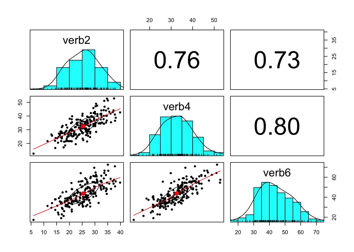
For clarity, let’s consider the basic information representation of the 3-occasion repeated measures data. In particular, data (even non-repeated measures data) are summarized (at the sample-level) as (1) a vector of means and (2) a variance-covariance matrix.

#mean vector (from wide data)
meanvector <- sapply(wiscsub[ ,c("verb2","verb4","verb6")], mean, na.rm=TRUE)
round(meanvector,2)

## verb2 verb4 verb6 
## 25.42 32.61 43.75

#variance-covariance matrix (from wide data)
varcovmatrix <- cov(wiscsub[ ,c("verb2","verb4","verb6")], use="pairwise.complete.obs")
round(varcovmatrix,2)

##       verb2 verb4  verb6
## verb2 37.29 33.82  47.40
## verb4 33.82 53.58  62.25
## verb6 47.40 62.25 113.74

Making visual counterparts can also be extremely useful - especially for facilitating higher-level conversations in a research group. Basic sample-level descriptions in visual form. Note that the time variable has been converted to a factor = categorical

ggplot(data=verblong, aes(x=factor(grade), y=verb)) + 
  geom_boxplot(notch = TRUE) +
  stat_summary(fun.y="mean", geom="point", shape=23, size=3, fill="white") +
  labs(x = "Grade", y = "Verbal Ability") +
  theme_classic()

## Warning: The `fun.y` argument of `stat_summary()` is deprecated as of ggplot2 3.3.0.
## ℹ Please use the `fun` argument instead.
## This warning is displayed once every 8 hours.
## Call `lifecycle::last_lifecycle_warnings()` to see where this warning was
## generated.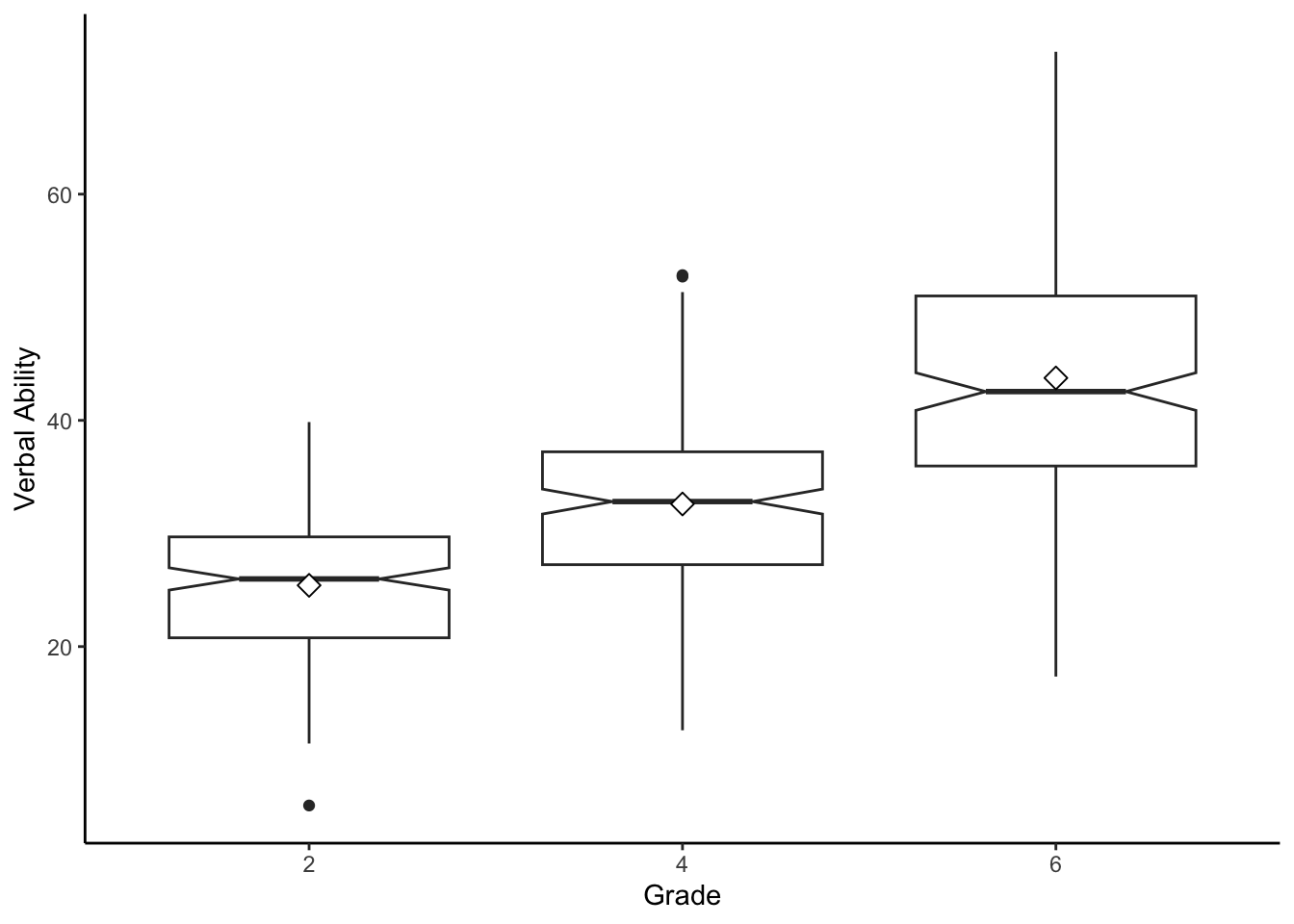

pairs.panels(wiscsub[,c("verb2","verb4","verb6")])

Reminder, we should always be careful about the scaling of the x- and y-axes in these plots.

One additional recoding for convenience is to center and scale our time variable. This gives us a specific \(0\) point and an intuitive \(0, 1, 2\) scale that is useful for our didactic purposes.

unique(verblong$grade)

## [1] 2 4 6

verblong$time0 <- (verblong$grade-2)/2 # from 2,4,6 to 0,1,2
unique(verblong$time0)

## [1] 0 1 2

head(verblong,12)

##     id grade  verb grad time0
## 1.2  1     2 26.98    0     0
## 1.4  1     4 39.61    0     1
## 1.6  1     6 55.64    0     2
## 2.2  2     2 14.38    0     0
## 2.4  2     4 21.92    0     1
## 2.6  2     6 37.81    0     2
## 3.2  3     2 33.51    1     0
## 3.4  3     4 34.30    1     1
## 3.6  3     6 50.18    1     2
## 4.2  4     2 28.39    1     0
## 4.4  4     4 42.16    1     1
## 4.6  4     6 44.72    1     2

Plotting the raw data along this new time variable.

#plotting intraindividual change RAW DATA
ggplot(data = verblong, aes(x = time0, y = verb, group = id)) +
  ggtitle("Raw Data") +
  geom_point() + 
  geom_line() +
  xlab("Time") + 
  ylab("WISC Verbal Score") + 
  ylim(0,100) + xlim(0,2) +
  theme_classic()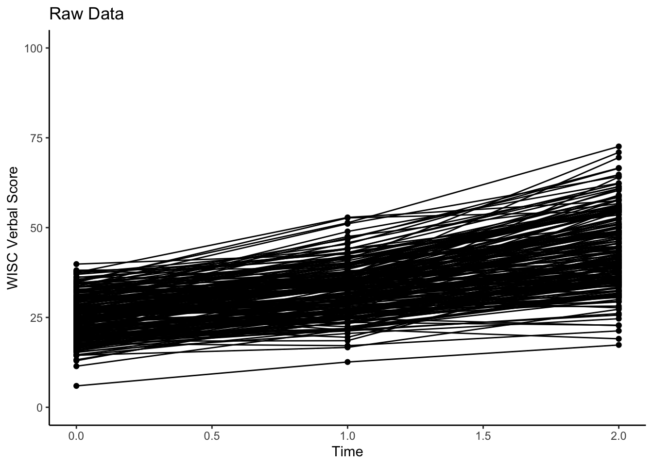

Note that the time variable in this plot has NOT been converted to a factor. It is a continuous variable.