5.3 Assumptions of OLS
The assumptions of OLS are as follows:
- \(\mathbb{E}(\epsilon_{i}) = 0\)
- \(\mathbb{E}(\epsilon_{i}^2) = \sigma^2\) for all \(i\) (homoscedasticity)
- \(\mathbb{E}(\epsilon_{i}\epsilon_{j}) = 0\) for all \(i \neq j\)
- No perfect collinearity among \(x\) variables
- \(\mathbb{C}(\epsilon_{i},x_{qi}) = 0\) for all \(i\) and \(k\)
Let’s discuss each assumption in more detail.
5.3.1 Assumption 1. \(\mathbb{E}(\epsilon_{i}) = 0\)
Note that \(\mathbb{E}()\) is the expectation operator. The expected value is an “average” of whatever is inside the parentheses. This assumption states that, on average, the error for the \(ith\) observation is zero. Here “for all \(i\)” means the same is true for all cases.
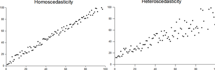
5.3.2 Assumption 2. Homoscedasticity
In statistics, a vector of random variables is heteroscedastic if the variability of the random disturbance is different across elements of the vector, here our \(\mathbf{X}\)s. The errors or disturbances in our model are homoskedastic if the variance of \(\epsilon _{i}\) is a constant (e.g. \(\sigma ^{2}\)), otherwise, they are heteroskedastic.
Graphical Depiction of Homoskedasticity and Heteroskedasticity
5.3.3 3. \(\mathbb{E}(\epsilon_{i}\epsilon_{j}) = 0\)
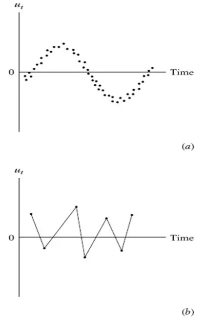
Assumption 3 is sometimes referred to as the autocorrelation assumption. This assumption states that the error terms of different observations should not be correlated with each other. For example, when we have time series data and use lagged variables we may want to examine residuals for the possibility of autocorrelation.
Graphical Depiction of Positive and Negative Autocorrelation
5.3.4 4. No Perfect Collinearity
Perfect collinearity occurs when one variable is a perfect linear function of any other explanatory variable. If perfect collinearity is found among the \(\mathbf{X}\)s then \(\mathbf{(X'X)}\) has no inverse and OLS estimation fails. Perfect collinearity is unlikely except for programming mistakes such as dummy coding all the values in a nominal variable.
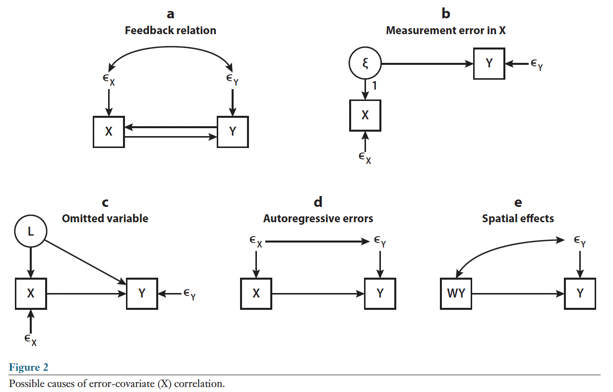
5.3.5 5. \(\mathbb{C}(\epsilon_{i},x_{ki}) = 0\)
Note that \(\mathbb{C}()\) is the covariance operator. Assumption five states that that the error of our equation is uncorrelated with all the \(\mathbf{X}\)s. This is often referred to as an endogeneity assumption.
This can be a confusing assumption because by definition the residuals \(\hat{e_i}\) are uncorrelated with the \(\mathbf{X}\)s. Here, however, we are concerned with the true errors \(\epsilon_i\). Unfortunately, there are a variety of conditions that lead to \(\mathbb{C}(\epsilon_{i},x_{qi}) \neq 0\) in applied contexts.
Graphical Depiction of Sources of Endogeneity
If we meet these assumptions what large sample properties can we expect?