11.10 Example Data III

Consider a second example dataset, where, again

We have an equal number of dyads that did and did not cohabit
Cohabitation had a null effect on changes in relationship satisfaction.
Dyads did not exhibit any changes in relationship satisfaction over time.

Unlike the first dataset, however, this second dataset would have been obtained if Sofia could have randomly assigned dyads to cohabit or live apart.

This second data set is in line with the assumption of the residualized change model, where the Time 1 score is uncorrelated with the key predictor, which is equivalent to affirming there are no preexisting group differences at baseline; there is one population of dyads at baseline with respect to relationship satisfaction.

11.10.1 Generate Some Data According to (Castro-Schilo and Grimm 2018) Example B

# set a seed so we all have the same data
set.seed (1234)

# create an id variable (N = 100 in each group)
id <- c(1:100, 1:100)

# create a time variable (0 = time 1, 1 = time 2)
time <- c(rep(0, 100), rep(1, 100))

# create grouping variable with equal number cohabiting (1) and not (0)
cohabit <- rep(c(0,1), 100)

# put all variables in a dataframe
data <- data.frame(id, cohabit, time)

# generate dataset A
data_B <- data
data_B$score <- 
  4.5 +                          # intercept
  0*data_B$cohabit +            # difference in cohabitation
  0*data_B$time +                # effect of time
  0*data_B$cohabit*data_B$time + # interaction
  rnorm(200, 0, 0.3)             # error


# Make into wide format for computing difference score
data_B <- reshape(
  data_B, 
  v.names = 'score', 
  timevar = "time",
  idvar = "id", 
  direction= "wide"
)

# assign appropriate variable names
names(data_B) <- c('id', 'cohabit', 'score1', 'score2')

# compute difference variable
data_B$diff <- data_B$score2 - data_B$score1

# declare cohabiting variable as a factor (categorical variable)
data_B$cohabit <- factor(data_B$cohabit)

11.10.2 Plot Data

# visualize the data
library(ggplot2)
ggplot(data_B, aes(x = score1, y = score2, shape= cohabit)) + 
  geom_point(size = 3) +
  geom_smooth(method = lm, se = F) +
  xlab("Relationship Satisfaction Time 1") +
  ylab("Relationship Satisfaction Time 2")

## `geom_smooth()` using formula = 'y ~ x'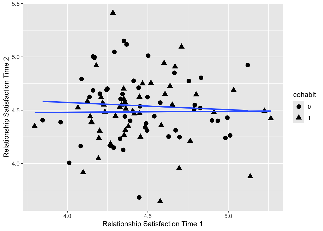

11.10.3 Fit Residualized Change Model

# ancova model
mylml <- lm(score2 ~ score1 + cohabit, data = data_B)
summary (mylml)

## 
## Call:
## lm(formula = score2 ~ score1 + cohabit, data = data_B)
## 
## Residuals:
##      Min       1Q   Median       3Q      Max 
## -0.86084 -0.17640  0.00684  0.17019  0.92449 
## 
## Coefficients:
##             Estimate Std. Error t value Pr(>|t|)    
## (Intercept)  4.66901    0.46562  10.028   <2e-16 ***
## score1      -0.02875    0.10390  -0.277    0.783    
## cohabit1    -0.05724    0.06230  -0.919    0.361    
## ---
## Signif. codes:  0 '***' 0.001 '**' 0.01 '*' 0.05 '.' 0.1 ' ' 1
## 
## Residual standard error: 0.3114 on 97 degrees of freedom
## Multiple R-squared:  0.009265,   Adjusted R-squared:  -0.01116 
## F-statistic: 0.4535 on 2 and 97 DF,  p-value: 0.6367

11.10.4 Fit Difference Score Model

# difference model
mylm2 = lm(diff ~ cohabit, data = data_B)
summary(mylm2)

## 
## Call:
## lm(formula = diff ~ cohabit, data = data_B)
## 
## Residuals:
##      Min       1Q   Median       3Q      Max 
## -1.29920 -0.22982  0.00904  0.28891  1.09081 
## 
## Coefficients:
##             Estimate Std. Error t value Pr(>|t|)
## (Intercept)  0.07941    0.06212   1.278    0.204
## cohabit1    -0.04002    0.08786  -0.455    0.650
## 
## Residual standard error: 0.4393 on 98 degrees of freedom
## Multiple R-squared:  0.002113,   Adjusted R-squared:  -0.00807 
## F-statistic: 0.2075 on 1 and 98 DF,  p-value: 0.6498

References

Castro-Schilo, Laura, and Kevin J Grimm. 2018. “Using Residualized Change Versus Difference Scores for Longitudinal Research.” Journal of Social and Personal Relationships 35 (1): 32–58.