6.6 Categorical Variable Interaction
Ok, let’s move on to the topic of an interaction which uses the product of two predictor variables as a new predictor.
Working up a slightly different example with the ‘grad’ variable (whether dad graduated high school),
\[ verb_{2i} = b_01_i + b_1verb^{*}_{1i} + b_2grad_{i} + b_3(verb^{*}_{1i}grad_{i}) + \epsilon_{i}\]
Where \(verb^{*}_{1i}\) is the mean-centered version of \(verb_{1i}\), and \(grad_i\) is a dummy coded variable that equals 0 if the child’s father did not graduate high school, and equals 1 if the child’s father did graduate high school.
We did not sample-mean center \(grad_i\) in this example because a value of 0 already has substantive meaning for the current example (i.e. when \(grad_i\) equals 0, the father did not graduate high school).
6.6.1 Interaction as Moderation
Often, we describe phenomena in terms of moderation; or that the relation between two variables (i.e. \(y_i\) and \(x_{1i}\)) is moderated by a third variable (i.e. \(x_{2i}\)). For example, the relation between Grade 1 and Grade 2 verbal scores may be moderated by father’s graduation status. More specifically, the relation between 1st and 2nd grade verbal score may be different for children whose fathers’ did not or did graduate from high school.
The inclusion of product terms (i.e. interactions) allows for a direct investigation of a moderation hypothesis.
6.6.2 Moderation by Categorical Variable
When the moderator is a dummy variable then the form of the moderation becomes fairly simple; we will have one equation for \(grad_{i} = 0\), and a second equation for \(grad_i = 1\).
6.6.2.1 Rewriting Equation
To illustrate the notion of two equations, let’s rewrite the regression equation
\[ verb_{2i} = b_01_i + b_1verb^{*}_{1i} + b_2grad_{i} + b_3(verb^{*}_{1i}grad_{i}) + \epsilon_{i}\]
as two separate regression equations, one for fathers who graduated from highschool and one for fathers that did not. We can accomplish this by plugging in \(0\) and \(1\) into the regression equation and rearranging some of the terms. Doing so we get
Equation for Students whose father Graduated Highschool
\[ verb_{2i} = (b_0 + b_2) + (b_1 + b_3)verb^{*}_{1i} + \epsilon_{i}\]
Equation for Students whose father Did Not Graduate from Highschool
\[ verb_{2i} = b_0 + b_1verb^{*}_{1i} + \epsilon_{i}\]
6.6.3 Interpretation
Without an interaction, our linear regression model assumes that the only difference between the regression line for each group (graduate HS vs not) is the intercept. That is, it assumes that the relationship between verbal scores at Grades 1 and 2 is the same for both groups.
Children Whose father’s Did Not Graduate HS
The expected Grade 2 verbal score for a child whose father did not graduate high school and who had an average Grade 1 verbal score is \(b_0\). Also, for a child whose father did not graduate high school, \(b_1\) is the expected difference in their Grade 2 verbal score for a one-point difference in their Grade 1 verbal score.
Children Whose father’s Did Not Graduate HS
The parameter estimates \(b_0\) and \(b_1\) maintain their interpretation from before. But now each of them is moderated (i.e. shifted or altered) by \(b_2\) or \(b_3\).
Specifically, the expected Grade 2 verbal score for a child whose father did graduate high school and who earned an average Grade 1 verbal score is \(b_0 + b_2\).
And, for a child whose father did graduate high school, \(b_1 + b_3\) is the expected difference in their Grade 2 verbal score for a one-point change in their Grade 1 verbal score.
6.6.4 Fit Regression Model in R
OK - let’s fit the model! Note that within this model we use the code I(verb1_star * grad). This produces the interaction term within the model. The wrapper function I() indicates to R to perform this data computation as-is, otherwise we would need to perform this computation (i.e. the multiplication of verb1_star by grad) outside of the function lm().
model5 <- lm(verb2 ~ 1 + verb1_star + grad + I(verb1_star*grad),
              data = wiscsub,
              na.action = na.exclude)
summary(model5)
##
## Call:
## lm(formula = verb2 ~ 1 + verb1_star + grad + I(verb1_star * grad),
## data = wiscsub, na.action = na.exclude)
##
## Residuals:
## Min 1Q Median 3Q Max
## -11.3433 -3.0761 -0.0825 2.5689 10.7289
##
## Coefficients:
## Estimate Std. Error t value Pr(>|t|)
## (Intercept) 25.2663 0.3416 73.956 <2e-16 ***
## verb1_star 0.7861 0.0604 13.015 <2e-16 ***
## grad 1.4632 0.8107 1.805 0.0726 .
## I(verb1_star * grad) -0.2430 0.1324 -1.836 0.0678 .
## ---
## Signif. codes: 0 '***' 0.001 '**' 0.01 '*' 0.05 '.' 0.1 ' ' 1
##
## Residual standard error: 4.232 on 200 degrees of freedom
## Multiple R-squared: 0.5268, Adjusted R-squared: 0.5197
## F-statistic: 74.22 on 3 and 200 DF, p-value: < 2.2e-166.6.5 Path Diagram

The parameter estimates from this model indicate that, for children whose father did not graduate high school, the expected Grade 2 verbal score for a child that earned an average 1st grade verbal score equals 25.2663 (\(b_0\)).
Also, for children whose father did not graduate high school, a 1-point difference in their Grade 1 verbal score is expected to correspond with a 0.7861 (\(b_1\)) point difference in the Grade 2 verbal score.
Moreover, the parameter estimates indicate that, for children whose father did graduate high school, the expected Grade 2 verbal score for a child that earned an average Grade 1 verbal score is 25.2663 + 1.4632 = 26.7295 (\(b_0 + b_2\)).
Also, for children whose father graduated high school, a 1-point difference in their Grade 1 verbal score is expected to correspond with a (\(b_1 + b_3\)) = 0.7861 - 0.2430 = 0.5431 point difference in the Grade 2 verbal score.
Even though the interaction is not significant, we can plot it for illustrating the moderation effect:
#plot of moderation
ggplot(data=wiscsub,
       aes(y=verb2,x=verb1_star, color = factor(grad))) +
  geom_jitter() +
  stat_smooth(method='lm', se=TRUE, fullrange=TRUE) +
  xlab("1st Grade Verbal Score") +
  ylab("2nd Grade Verbal Score") +
  guides(color=guide_legend(title="HS Grad")) +
  theme_bw()
## `geom_smooth()` using formula = 'y ~ x'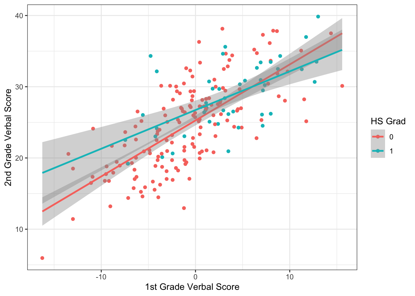
The example from ‘model5’ contained an interaction using a dummy variable (i.e., \(grad_i\)). Interactions may also occur between two continuous variables (i.e., \(verb^{*}_{1i}\) and \(daded^{*}_{i}\)). We will not cover here, but note that it is still very useful to consider and communicate those interactions as moderation. There are many resources on interactions of two (or more) continuous variables.